Problem Set 4

Data analysis and machine learning

Due date: 2021-03-25 17:00 (Melbourne time) unless by prior arrangement

Your submission should be in the form of a PDF that includes relevant figures. The PDF can be compiled from $\LaTeX$ or outputted by Jupyter notebook, or similar. You must also submit code scripts that reproduce your work in full.

Marks will depend on the results/figures that you produce, and the clarity and depth of your accompanying interpretation. Don't just submit figures and code! You must demonstrate understanding and justification of what you have submitted. Please ensure figures have appropriate axes, that you have adopted sensible mathematical nomenclature, et cetera.

\[ \newcommand{\transpose}{^{\scriptscriptstyle \top}} \newcommand{\vec}[1]{\mathbf{#1}} \]

In total there are 2 questions in this problem set, with a total of 30 marks available.

Question 1

(Total 10 marks available)

Define and explain the following terms in machine learning. You may provide equations or example figures to aid your explanation.

Precision
Recall
F1 score
Regularisation, including LASSO and Ridge regression
Confusion matrices

Question 2

(Total 20 marks available)

(This question requires you to install the scikit-learn Python package.)

You are tasked with performing dimensionality reduction on a set of images of human faces. In this question you will use an existing package to do the PCA for you. Remember that if you were to do this yourself, your data must be mean-centered and unit variance in every dimension before you do PCA!

from sklearn.datasets import fetch_lfw_people faces = fetch_lfw_people(min_faces_per_person=50) # Who are these people?! print(faces.target_names) ['Ariel Sharon' 'Colin Powell' 'Donald Rumsfeld' 'George W Bush' 'Gerhard Schroeder' 'Hugo Chavez' 'Jacques Chirac' 'Jean Chretien' 'John Ashcroft' 'Junichiro Koizumi' 'Serena Williams' 'Tony Blair'] # What do their faces look like? print(faces.images.shape) (1560, 62, 47) # The target name index for each image (0 = Ariel Sharon, etc) print(faces.target.shape) 1560 print(faces.target) [11, 4, 2, ..., 3, 11, 5]

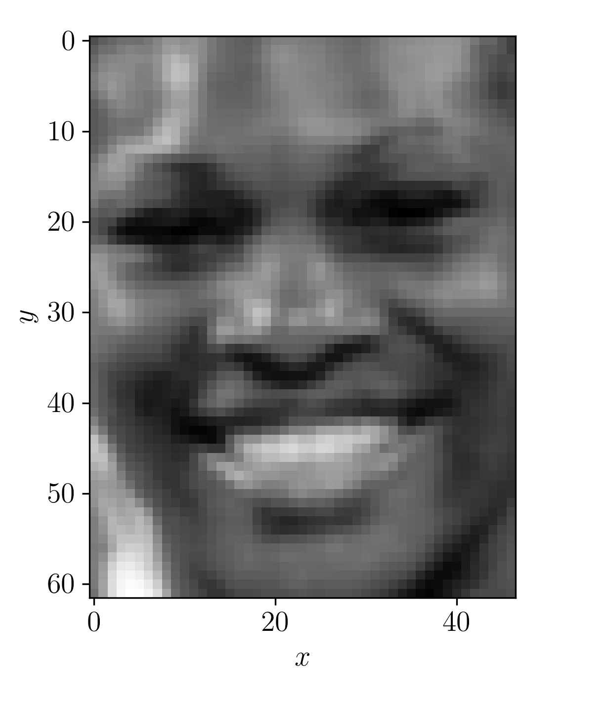
You can see that we have 1,560 images, where each image is 62 pixels by 47 pixels. Let's plot an image. import matplotlib.pyplot as plt fig, ax = plt.subplots(figsize=(4, 4.75)) ax.imshow(faces.images[12], cmap="binary_r") ax.set_xlabel(r"$x$") ax.set_ylabel(r"$y$") fig.tight_layout()

Serena Williams is better at tennis than you and me.

Task one

Use PCA to fit these images (sklearn.decomposition.PCA) and find the first 150 principal components. You will find that the dimensionality of this data is large, so vanilla PCA will have a hard time. Use the 'random' algorithm as the SVD solver, which takes random subsets of the data to find the first $N$ components. Make a figure showing the first 50 components (eigenfaces) as images, with one image per panel. This code example might help you set up your figure:

fig, axes = plt.subplots(5, 10, figsize=(10, 5), subplot_kw={'xticks':[], 'yticks':[]}, gridspec_kw=dict(hspace=0.1, wspace=0.1)) for i, ax in enumerate(axes.flat): # plot things to ax

Task two

Plot the cumulative explained variance as a function of the number of principal components.

Task three

Use PCA to compute the contributions from the first 150 principal components for every data point. You should have an array that is 1,560 by 150 (the number of images by the number of components). Now use these components to take an inverse transform with PCA, to show projected images using only those 150 components. For each person in the data set, plot an original image of them compared to the reconstructed image using 150 principal components.