\[
\newcommand{\transpose}{^{\scriptscriptstyle \top}}
\newcommand{\vec}[1]{\mathbf{#1}}
\]
In total there are six questions in this problem set, with a total of 60 marks available.
Question 1
(Total 10 marks available)
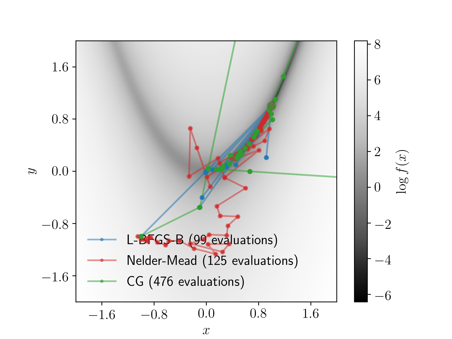
Rosenbrock's function is
\[
f(x, y) = (1 - x)^2 + 100(y - x^2)^2 \quad .
\]
Calculate \(\log{f(x,y)}\) on a grid of \(x\) and \(y\) values from \(x \in [-2, 2]\) and \(y \in [-2, 2]\) with 250 grid points in each direction. Plot the \(\log{f(x,y)}\) contours and include a colour bar to show the value of \(\log{f(x,y)}\).
Starting from an initial value of \((x,y) = (-1, -1)\), find the minima given by Rosenbrock's function using
- the BFGS (or L-BFGS-B) algorithm,
- the Nelder-Mead algorithm (also known as the simplex algorithm), and
- an algorithm of your choice.
For each algorithm, record the \((x,y)\) points trialled by the algorithm and plot these on the figure you have made. This will show the path of both optimisation algorithms. Be sure to include a legend so it is clear which path corresponds to which algorithm.
Hot Tip: You can record the positions trialled by an optimisation algorithm using an example like this:
import numpy as np
import scipy.optimize as op
# Let's define a list to store the positions in.
positions = []
# Define the objective function.
def objective_function(theta):
positions.append(theta)
x, y = theta
# Remember: you have to write your own `rosenbrocks` function
return rosenbrocks(x, y) # or just rosenbrocks(*theta)
op_result = op.minimize(
objective_function,
[-1, 1],
method="Nelder-Mead"
)
# Now let's use the recorded positions.
positions = np.array(positions)
Solution
import numpy as np
import matplotlib.pyplot as plt
import scipy.optimize as op
from matplotlib.ticker import MaxNLocator
def rosenbrock(x, y):
return (1 - x)**2 + 100*(y - x**2)**2
bins = 250
x_bounds = (-2, 2)
y_bounds = (-2, 2)
x_bins = np.linspace(*x_bounds, bins)
y_bins = np.linspace(*y_bounds, bins)
X, Y = np.meshgrid(x_bins, y_bins)
F = np.log(rosenbrock(X, Y))
imshow_kwds = dict(
origin="lower",
extent=(*x_bounds, *y_bounds),
aspect=np.ptp(x_bounds)/np.ptp(y_bounds)
)
fig, ax = plt.subplots()
image = ax.imshow(
F,
cmap="Greys_r",
**imshow_kwds
)
cbar = plt.colorbar(image)
cbar.set_label(r"$\log{f(x)}$")
ax.set_xlabel(r"$x$")
ax.set_ylabel(r"$y$")
ax.xaxis.set_major_locator(MaxNLocator(6))
ax.yaxis.set_major_locator(MaxNLocator(6))
# Initialise
initial_theta = [-1, -1]
methods = [
("L-BFGS-B", "tab:blue", dict(epsilon=1e-8)),
("Nelder-Mead", "tab:red", None),
("CG", "tab:green", None)
]
for method, color, options in methods:
positions = []
def objective_function(theta):
positions.append(theta)
print(theta)
return rosenbrock(*theta)
op_result = op.minimize(
objective_function,
initial_theta,
method=method,
options=options
)
positions = np.array(positions)
ax.plot(
*positions.T,
c=color,
alpha=0.5,
label=f"{method} ({len(positions)} evaluations)"
)
ax.scatter(
[positions.T[0]], [positions.T[1]],
facecolor=color,
s=10, zorder=50, alpha=0.5
)
ax.scatter(
[op_result.x[0]], [op_result.x[1]],
facecolor=color,
s=50, zorder=100, alpha=0.5
)
ax.legend(frameon=False)
Question 2
(Total 5 marks available)
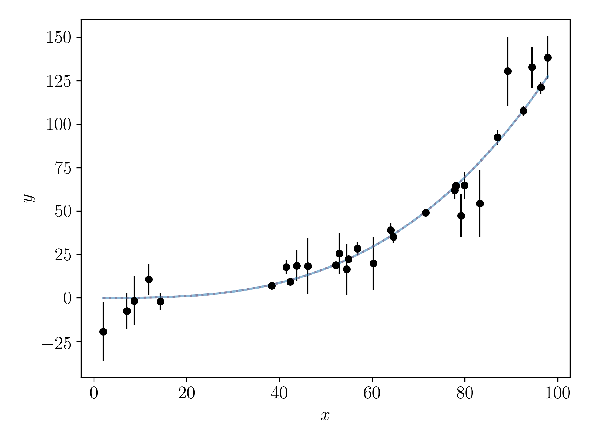
Use the following code to generate some fake data that are drawn from the model
\[
y \sim \mathcal{N}\left(\theta_0 + \theta_1x + \theta_2x^2 + \theta_3x^3,\sigma_{y}\right)
\]
import numpy as np
np.random.seed(0)
N = 30
x = np.random.uniform(0, 100, N)
theta = np.random.uniform(-1e-3, 1e-3, size=(4, 1))
# Define the design matrix.
A = np.vstack([
np.ones(N),
x,
x**2,
x**3
]).T
y_true = (A @ theta).flatten()
y_err_intrinsic = 10 # MAGIC number!
y_err = y_err_intrinsic * np.random.randn(N)
y = y_true + np.random.randn(N) * y_err
y_err = np.abs(y_err)
Even though this model includes \(x^2\) and \(x^3\) terms, this is still a linear problem that you can solve with linear algebra! Do you see why that is? (This is the generalised representation of ordinary least-squares!)
Let us assume that the generated data have no uncertainties in the \(x\)-direction, and that the uncertainties in the \(y\)-direction are normally distributed. Cast this problem with matrices and find a point estimate of the best-fitting model parameters. Make a plot showing the data, the true model, and the model using the best-fitting model parameters.
Solution
np.random.seed(0)
N = 30
x = np.random.uniform(0, 100, N)
D = 4
X = np.random.uniform(-1e-3, 1e-3, size=(D, 1))
# Define the design matrix.
A = np.vstack([
np.ones(N),
x,
x**2,
x**3
]).T[:, :D]
Y = A @ X
y_true = Y.flatten()
y_err_intrinsic = 10
y_err = y_err_intrinsic * np.random.randn(N)
y = y_true + np.random.randn(N) * y_err
y_err = np.abs(y_err)
fig, ax = plt.subplots()
ax.scatter(x, y, c="k", s=10)
ax.errorbar(x, y, yerr=y_err, fmt="o", lw=1, c="k")
# Find some estimate of the best values.
C_inv = np.eye(N) * y_err**-2
# X_hat = (A.T C^{-1} A)^{-1} (A.T C^{-1} Y)
X_hat = np.linalg.inv(A.T @ C_inv @ A) @ (A.T @ C_inv @ Y)
xi = np.linspace(x.min(), x.max(), 1000)
yi = np.polyval(X_hat[::-1], xi)
ax.plot(xi, yi, c="tab:red", ls=":", alpha=0.5)
ax.plot(xi, np.polyval(X.flatten()[::-1], xi), c="tab:blue", ls="-", alpha=0.5)
ax.set_xlabel(r"$x$")
ax.set_ylabel(r"$y$")
fig.tight_layout()
Question 3
(Total 10 marks available)
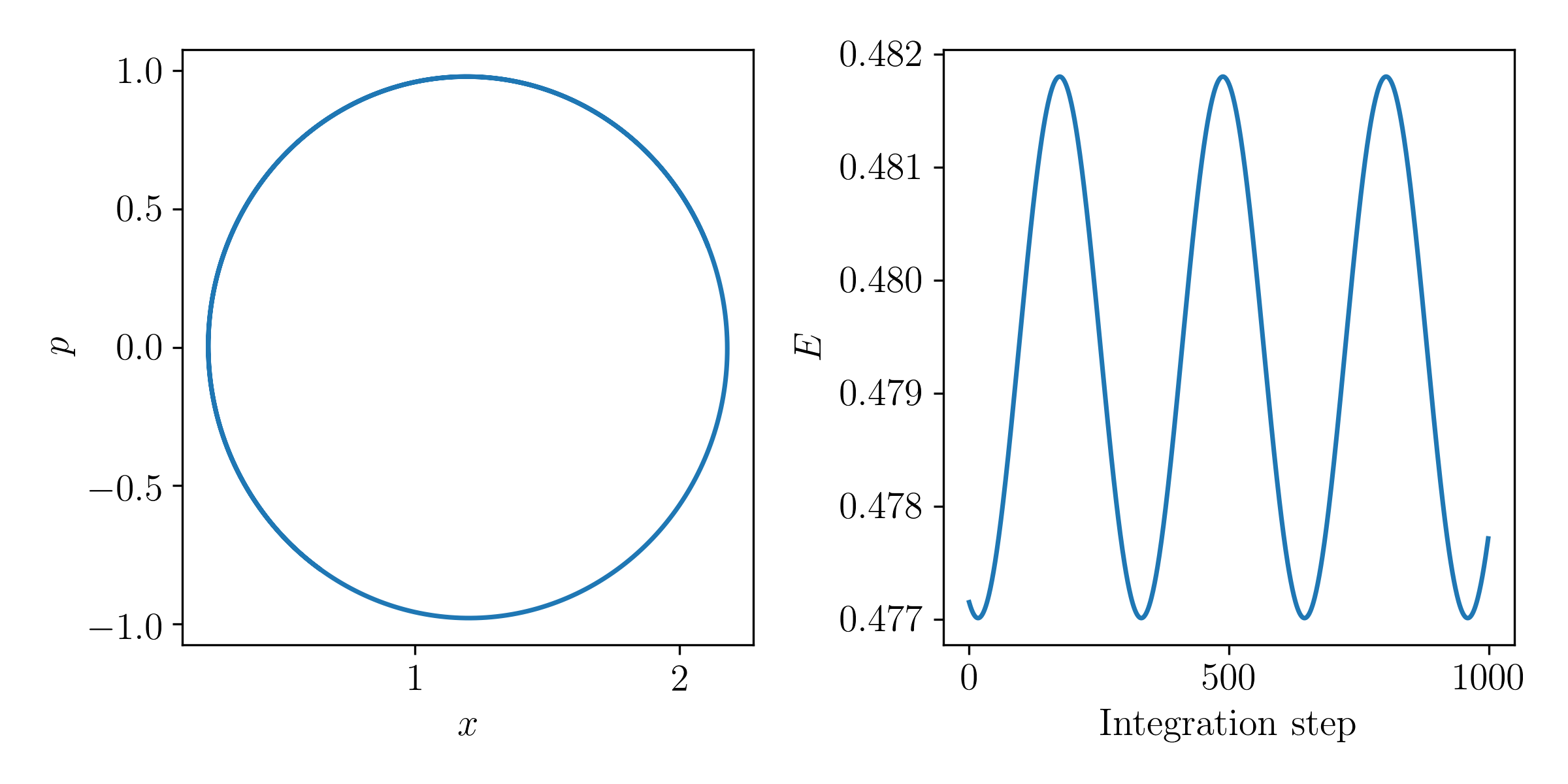
In this question we will use a Leapfrog integrator to integrate the motion of a particle in a potential.
This will be used in Question 4 when you implement a Hamiltonian Monte Carlo sampler. Recall that at time \(t\) a particle in some system with a location \(\vec{x}(t)\) and a momentum \(\vec{p}(t)\) can be fully described by the Hamiltonian
\[
\mathcal{H}\left(\vec{x},\vec{p}\right) = U\left(\vec{x}\right) + K\left(\vec{p}\right)
\]
where the sum of gravitational \(U\) and kinetic \(K\) energy remains constant with time. Let
\[
K(\vec{p}) = \frac{\vec{p}\transpose\vec{p}}{2}
\]
and
\[
U(\vec{x}) = -\log{p(\vec{x})}
\]
where \(\log{p(\vec{x})}\) is short-hand notation for the log posterior probability for the model parameters \(\vec{x}\) (which we normally denote as \(\vec{\theta}\))
\[
\log{p(\vec{x})} \equiv \log{p(\vec{\theta}|\vec{y})} \quad .
\]
The time evolution of this particle is given by
\[
\frac{d\vec{x}}{dt} = \frac{\partial\mathcal{H}}{\partial\vec{p}} = \vec{p}
\]
and
\[
\frac{d\vec{p}}{dt} = -\frac{\partial\mathcal{H}}{\partial\vec{x}} = -\frac{\partial{}\log{p(\vec{x})}}{\partial{}\vec{x}} \quad .
\]
It is clear that that to integrate the motion of a particle in this system we will need the derivative of \(\log{p(\vec{x})}\) with respect to \(\vec{x}\).
Let us assume a model where we have a single data point \(y\) that is drawn from the model
\[
y \sim \mathcal{N}\left(y_t, \sigma_y\right)
\]
where our only model parameter is the true value \(y_t\). The single data point is \((y, \sigma_y) = (1.2, 1)\).
The negative log posterior probability function for this model can be written as:
def neg_log_prob(theta):
return 0.5 * (theta - 1.2)**2
Start with an initial guess of the model parameter somewhere between -1 and +1. Draw an initial momentum value \(p \sim \mathcal{N}(0, 1)\). With this initial position and momentum, integrate the orbit of the particle using a Leapfrog integration scheme. An example of the integration scheme is given below, but you will need to change this to record the particle position and momentum at every step. You will need the derivative of the log probability with respect to the parameters. Either derive this, or use JaxThe derivative here is easy to write down, but this is giving you the opportunity to learn about Jax, so that you are familiar with it when you move to more complex functions.:
from jax import grad
grad_neg_log_prob = grad(neg_log_prob)
Make a plot showing the particle position (x-axis) and its momentum (y-axis) at every step of the integrated orbit. In another plot, show the total energy of the system with each step. Is the energy conserved? Why or why not?
import numpy as np
def leapfrog_integration(x, p, dU_dx, n_steps, step_size):
"""
Integrate a particle along an orbit using the Leapfrog integration scheme.
"""
x = np.copy(x)
p = np.copy(p)
# Take a half-step first.
p -= 0.5 * step_size * dU_dx(x)
for step in range(n_steps):
x += step_size * p
p -= step_size * dU_dx(x)
x += step_size * p
p -= 0.5 * step_size * dU_dx(x)
return (x, -p)
Solution
from tqdm import tqdm
def leapfrog_integration(x, p, dv_dx, n_steps=100, step_size=1e-2, full_output=False):
"""
Integrate a particle along an orbit using the Leapfrog integration scheme.
"""
x = np.copy(x)
p = np.copy(p)
xs = np.empty(n_steps)
ps = np.empty(n_steps)
# Take a half-step first.
p -= 0.5 * step_size * dv_dx(x)
for step in range(n_steps):
x += step_size * p
p -= step_size * dv_dx(x)
xs[step] = x
ps[step] = p
x += step_size * p
p -= 0.5 * step_size * dv_dx(x)
# Flip the momentum to maintain detailed balance.
p = -p
if full_output:
return (x, p, xs, ps)
return (x, p)
def neg_log_prob(theta, **kwargs):
return 0.5 * np.sum((theta - 1.2)**2, **kwargs)
def grad_neg_log_prob(theta):
return theta - 1.2
np.random.seed(52)
D = 1
x = np.random.uniform(-1, 1, size=D)
p = np.random.normal(0, 1, size=D)
new_x, new_p, xs, ps = leapfrog_integration(x, p, grad_neg_log_prob, n_steps=1000, full_output=True)
fig, axes = plt.subplots(1, 2, figsize=(8, 4))
axes[0].plot(xs, ps, markersize=0)
axes[0].set_xlabel(r"$x$")
axes[0].set_ylabel(r"$p$")
# Calculate the total energy.
U = neg_log_prob(xs.reshape((-1, 1)), axis=1)
K = 0.5 * ps**2
E = U + K
axes[1].plot(E, markersize=0)
axes[1].set_xlabel(r"$\textrm{Integration~step}$")
axes[1].set_ylabel(r"$E$")
fig.tight_layout()
Question 4
(Total 15 marks available)
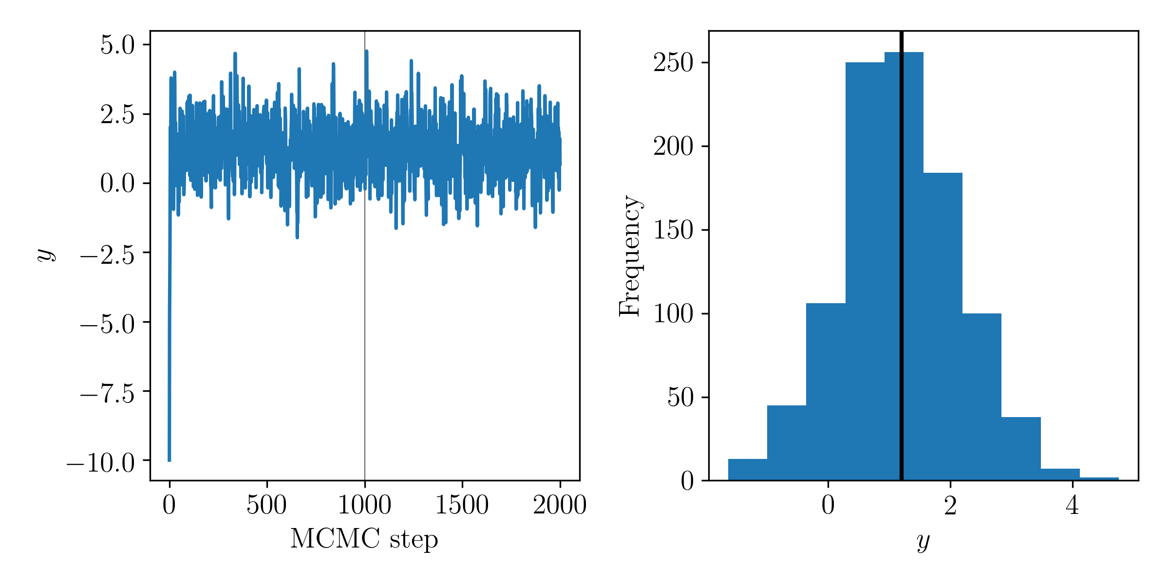
Use the potential and momentum distribution defined in Question 3 and build a Hamiltonian Monte Carlo sampler for the model defined in Question 3. Run your sampler for at least 1,000 steps, ensuring that you are taking appropriate number of steps (and step sizes) in the Leapfrog integration. Start the sampler from an initial value of \(x = -10\). Make a plot of the MCMC chain, and a histogram of the posterior on \(y_t\). Has the chain converged?
Solution
from scipy import stats
n_burn_in, n_production = (1000, 1000)
n_samples = n_burn_in + n_production
samples = [-10.0]
momentum = stats.norm(0, 1)
for p0 in tqdm(momentum.rvs(size=n_samples)):
new_x, new_p = leapfrog_integration(
samples[-1],
p0,
grad_neg_log_prob,
)
start_log_p = neg_log_prob(samples[-1]) - np.sum(momentum.logpdf(p0))
new_log_p = neg_log_prob(new_x) - np.sum(momentum.logpdf(new_p))
if np.log(np.random.rand()) < start_log_p - new_log_p:
samples.append(new_x)
else:
samples.append(np.copy(samples[-1]))
samples = np.array(samples)
fig, axes = plt.subplots(1, 2, figsize=(8, 4))
axes[0].plot(samples, markersize=0)
axes[0].set_xlabel(r"$\textrm{MCMC~step}$")
axes[0].set_ylabel(r"$y$")
axes[0].axvline(n_burn_in, c="#666666", lw=0.5, zorder=-1, markersize=0)
axes[1].hist(samples[n_burn_in:])
axes[1].set_xlabel(r"$y$")
axes[1].set_ylabel(r"$\textrm{Frequency}$")
axes[1].axvline(1.2, c="k", lw=2, markersize=0)
fig.tight_layout()
Question 5
(Total 10 marks available)
Implement the same model in Question 4 using PyMC or Stan. Use the default sampling algorithm and default hyperparameters to sample the posteriors. Make a plot showing the chains produced by your sampler and those from PyMC or Stan. Comment on any differences.
Solution
import stan
program_code = """
data {
real y;
real sigma;
}
parameters {
real y_t;
}
model {
y ~ normal(y_t, sigma);
}
"""
model = stan.build(program_code=program_code, data=dict(y=1.2, sigma=1))
stan_samples = model.sample(num_samples=500, num_chains=2)
fig, axes = plt.subplots(1, 2, figsize=(8, 4))
axes[0].plot(samples[n_burn_in:], c="tab:blue", markersize=0)
axes[0].plot(stan_samples["y_t"][0], c="tab:red", markersize=0)
axes[0].set_xlabel(r"$\textrm{MCMC~step}$")
axes[0].set_ylabel(r"$y$")
axes[1].set_xlabel(r"$y$")
axes[1].hist(
[samples[n_burn_in:], stan_samples["y_t"][0]],
color=("tab:blue", "tab:red"),
label=(r"$\textrm{Our~sampler}$", r"$\textrm{Stan}$"),
bins=30
)
fig.tight_layout()
axes[1].legend(loc="upper center", frameon=False, ncol=2)
axes[1].set_ylim(0, 140)
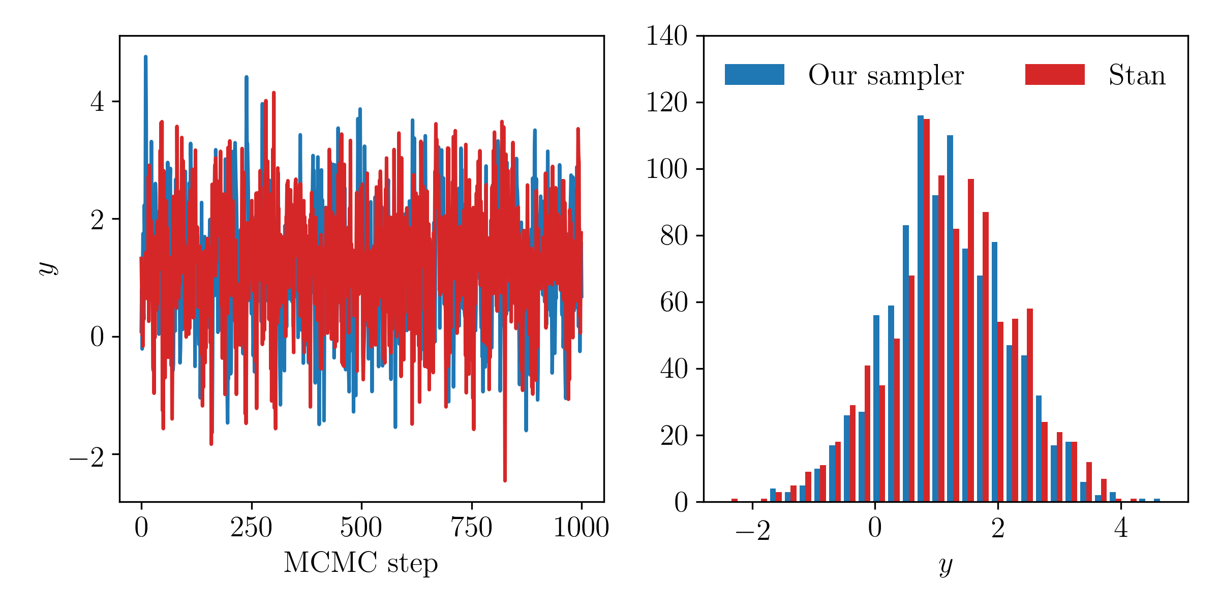
Our posterior samples agree excellently with those from Stan. If we had not set the step size of the Leapfrog integration scheme to be small enough, or had not taken enough Leapfrog steps, then these comparisons might look different.
Question 6
(Total 10 marks available)
Let us consider that we do not know what model truly generated the data in Question 2. Let's assume we think the data were generated by one of the following models:
\[
y = \theta_0 + \theta_1x
\]
\[
y = \theta_0 + \theta_1x + \theta_2x^2
\]
\[
y = \theta_0 + \theta_1x + \theta_2x^2 + \theta_3x^3
\]
\[
y = \theta_0 + \theta_1x + \theta_2x^2 + \theta_3x^3 + \theta_4x^4
\]
\[
y = \theta_0 + \theta_1x + \theta_2x^2 + \theta_3x^3 + \theta_4x^4 + \theta_5x^5
\]
\[
y = \theta_0 + \theta_1x + \theta_2x^2 + \theta_3x^3 + \theta_4x^4 + \theta_5x^5 + \theta_6x^6
\]
\[
y = \theta_0 + \theta_1x + \theta_2x^2 + \theta_3x^3 + \theta_4x^4 + \theta_5x^5 + \theta_6x^6 + \theta_7x^7
\]
For each model, find an estimate of the best model parameters. Make a plot showing the different models on the \(x\) axis, and the \(\log\mathcal{L}\) at the best model parameters for each model. From this figure, which model is best?
You want to calculate the evidence for each of these models, but you decide it is too much work to do for a single problem set. Instead, you decide to calculate the Bayesian Information Criteria (BIC) for each model. Plot the BIC for each model. From this metric, which model is best?
Comment on why BIC might be considered useful in this scenario, and why it may not be a good idea.
Solution
# Q6
np.random.seed(0)
N = 30
x = np.random.uniform(0, 100, N)
D = 4
X = np.random.uniform(-1e-3, 1e-3, size=(D, 1))
# Define the design matrix.
A = np.vstack([
np.ones(N),
x,
x**2,
x**3
]).T[:, :D]
Y = A @ X
y_true = Y.flatten()
y_err_intrinsic = 10
y_err = y_err_intrinsic * np.random.randn(N)
y = y_true + np.random.randn(N) * y_err
y_err = np.abs(y_err)
C_inv = np.diag(y_err**-2)
# Use linear algebra!
# X_hat = (A.T C^{-1} A)^{-1} (A.T C^{-1} Y)
def solve_system(max_polynomial_order):
N = Y.size
A = np.vstack(
[x**exponent for exponent in range(1 + max_polynomial_order)]
).T
X_hat = np.linalg.inv(A.T @ C_inv @ A) @ (A.T @ C_inv @ Y)
residual = (A @ X_hat - Y)
log_L = (-0.5 * residual.T @ C_inv @ residual).flatten()[0]
n_params = (max_polynomial_order + 1)
bic = n_params * np.log(N) - 2 * log_L
return (X_hat, log_L, bic)
bics = []
log_Ls = []
max_polynomial_orders = np.arange(1, 8)
for max_polynomial_order in max_polynomial_orders:
theta, log_L, bic = solve_system(max_polynomial_order)
log_Ls.append(log_L)
bics.append(bic)
fig, axes = plt.subplots(1, 2, figsize=(8, 4))
axes[0].plot(max_polynomial_orders, log_Ls, c="k", markersize=0)
axes[0].set_xlabel(r"$\textrm{Maximum~polynomial~order}$")
axes[0].set_ylabel(r"$\log{\hat{\mathcal{L}}}$")
axes[1].plot(max_polynomial_orders, bics, c="k", markersize=0)
axes[1].set_xlabel(r"$\textrm{Maximum~polynomial~order}$")
axes[1].set_ylabel(r"$\textrm{BIC}$")
# Mark best by BIC.
idx = np.argmin(bics)
axes[1].scatter([max_polynomial_orders[idx]], [bics[idx]], facecolor="k", s=10)
fig.tight_layout()
# Mark true
for ax in axes:
ax.axvline(3, c="#666666", lw=0.5, ls=":", zorder=-1, markersize=0)
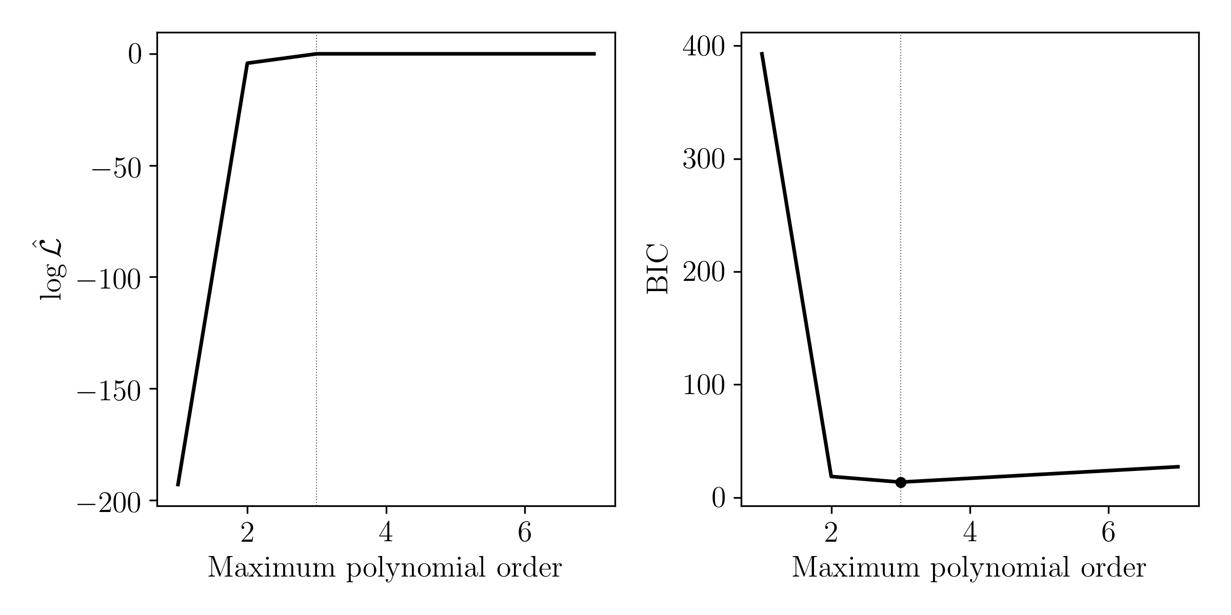
BIC is useful to approximate the normalisation constant between models from the same family. It does not account for any curvature in the log likelihood surface, so its applications are limited.