You will remember from Week 1 (Lecture 3) where you were already introduced to the concept of a mixture model. There we were saying that the data could be described as a mixture of two models: a straight line model describing some (unknown) fraction of the data, and a 'background' or 'outlier' model that described some (unknown) fraction of the data. This is an example of a mixture model!
To clarify the language it is worthwhile to state that: a mixture model is one where the data are described by a sum (or mixture) of multiple models. Usually when we are dealing with a mixture model we use the word component to specify one of the models in the mixture. For example, the model we adopted in Lecture 3 contains two components: a straight line component and a background component. Using the term 'component' helps us avoid overloading the term 'model'.
If we only have two components then things are easy, but mixture models can have more than two components. When there are many components involved, normally we are not referring to one component as being an "outlier" component or anything like that. In situations where there are many components we are simply saying that the data are drawn from a mixture of many components and our job as a data analyst would be
Let's consider the possibility that there is some data set that is described by \(K\) components
Remember here that we are not considering data points to have hard assignment in that the \(n\)-th data point 'belongs' to the k-th data point. Instead we are allowing for soft assignment where each data point will be described by some fraction of the components. You could have situations where the \(k\)-th component is almost entirely describing one data point in that the other components contribute \(1\times 10^{-10}\) to describing that data point, but we are still allowing for the possibility that each data point is described by a mixture of multiple components.
If you have any experience in clustering then you may have heard of mixture models before. Mixture models appear throughout all of data analysis and machine learning, and so we are going to use this lesson to tell you more about mixture models, and to introduce you to one of the most important algorithms in data analysis and machine learning: the expectation-maximization algorithm!
Optimising a mixture model
When we optimised the parameters for the mixture model described in Lecture 3 we didn't have to do anything special. We had one mixing proportion \(Q\), \[ Q \sim \mathcal{U}\left(0, 1\right) \] and we took \(1-Q\) as the mixing proportion for the outlier model. But when we have many components this becomes a non-trivial optimisation problem very quickly! Why do you think so?
One reason is obviously due to the non-convexity of the problem. Let's say we had one dimensional data that looks like this:
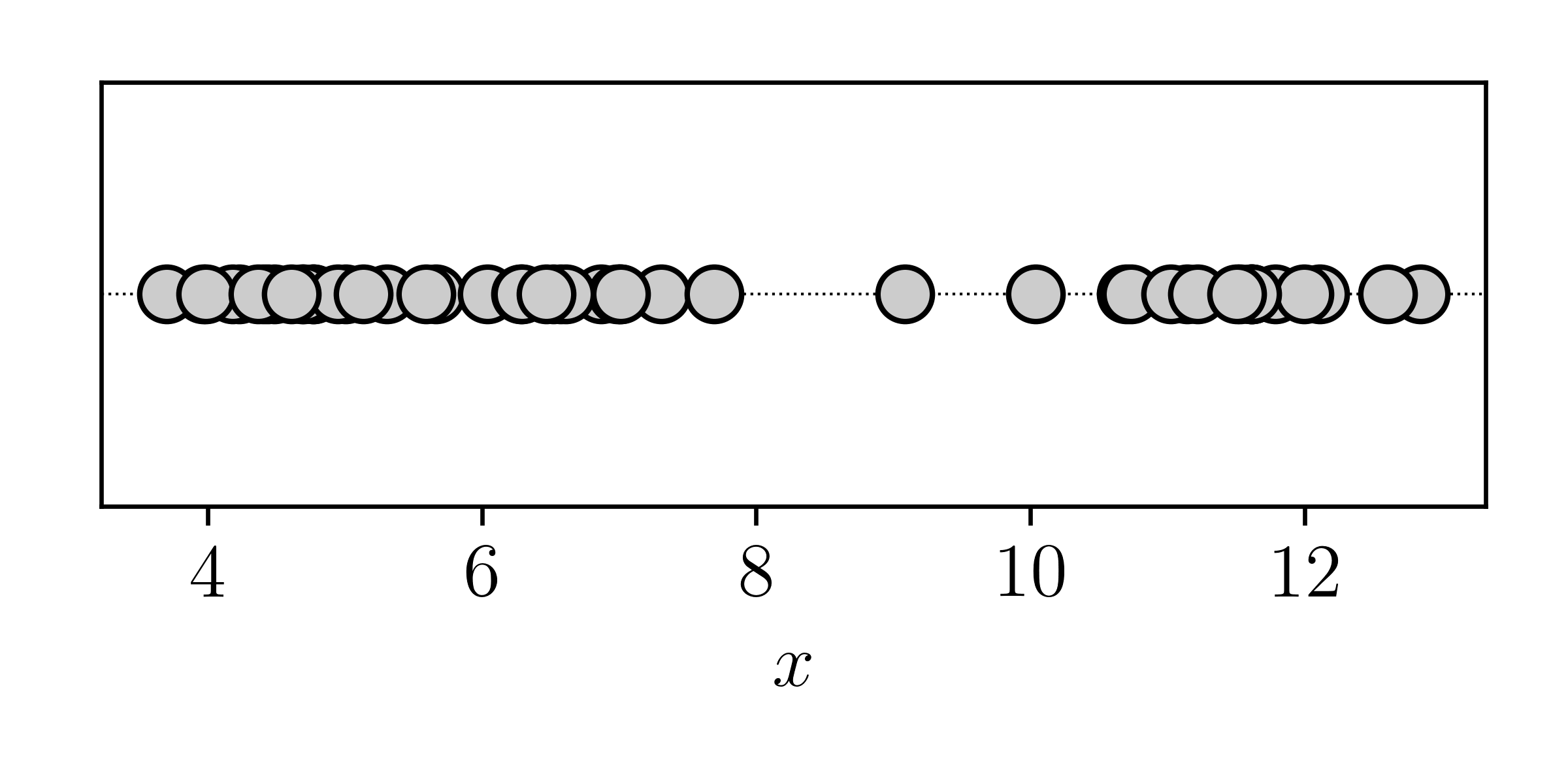
Let's say that these data are drawn from a mixture of three components, where each component is a Gaussian with some mean and some variance. We don't know what the means and variances are of any of the Gaussians. It is clear that if we were to treat this as a simple optimisation problem, there are a number of minima. For example, Component 1 could be the component with the mean and variance of the middle third of the data, or it could just as easily be the component describing the first third of the data. Or the last third!
This problem does become easier if you initialise the model parameters in a sensible way, but that only fixes the symptomns, not the underlying problem. The underlying problem will still have many equally-good minima. Strictly this is both an optimisation problem and an identifiability problem in that there is no mathematical constraint to state how the components should be ordered with respect to each other. Component 1 could describe the same data as Component 3 if you switched their means, variances, and mixing proportions!
There's another complication here too. Obviously each mixing proportion \(\pi_k\) will be bounded between zero and 1, \[ \pi_k \sim \mathcal{U}\left(0, 1\right) \] but there is the additional constraint that \(\sum^{K}\pi_k = 1\). To state this we can say \[ \pi \sim \textrm{Multinomial}(K) \] but we still have a problem in how to have each mixing proportion move in parameter space during optimisation.
While you can still solve this kind of mixture model problem with optimisation, in practice it can be numerically unstable or inefficient to do so using standard optimisation techniques. Instead we use something called the Expectation-Maximization approach.
Expectation-Maximization
Expectation-Maximization (E-M) is one of the simplest and most important algorithms in data analysis and machine learning. I find it best to explain E-M using a one dimensional data problem first, and then you will see how this generalises to multiple dimensions, and really to any problem. Expectation-Maximization is not just an ad-hoc method, in that it is built upon many elegant proofs, but we will leave those until the end.
OK, consider the data below:
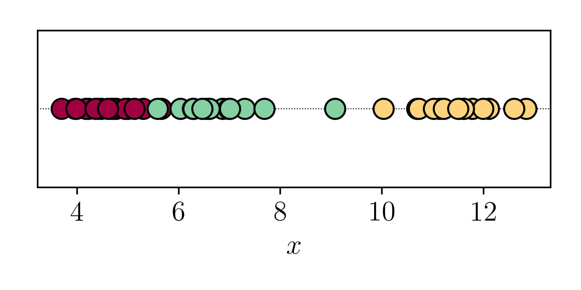
We are told that these data are drawn from three Gaussian components, and we are interested in inferring the parameters of those Gaussian components, and their mixing proportions. The parameters of each Gaussian component that we are interested in are the means and variances.
If we knew where each point came from..
Now imagine if we just knew which data point was drawn from what component.
If we knew this then estimating the means and variances for each component would be trivial! Let's say that Component A describes the red points, and then if we knew which points came from the red distribution we could just calculate the mean \[ \mu_1 = \frac{1}{N_\textrm{red}} \sum^{N_\textrm{red}}_{i=1} x_i \quad \textrm{for all red points} \] and variance \[ \sigma_1^2 = \frac{1}{N_\textrm{red}} \sum_{i=1}^{N_\textrm{red}} (x_i - \mu_1)^2 \] and we would already know the mixing proportion \(\pi_1\) \[ \pi_1 = \frac{N_\textrm{red}}{N} \] where \(N\) is the total number of data points. OK, so if we knew which data points were drawn from what component then it would be trivial to estimate the component parameters. But we don't normally know which data point came from what component!
If we knew the parameters of each component..
What if instead we tried to guess which data point came from what component? Let's try that, where we will start with some randomly chosen initial means and variances:
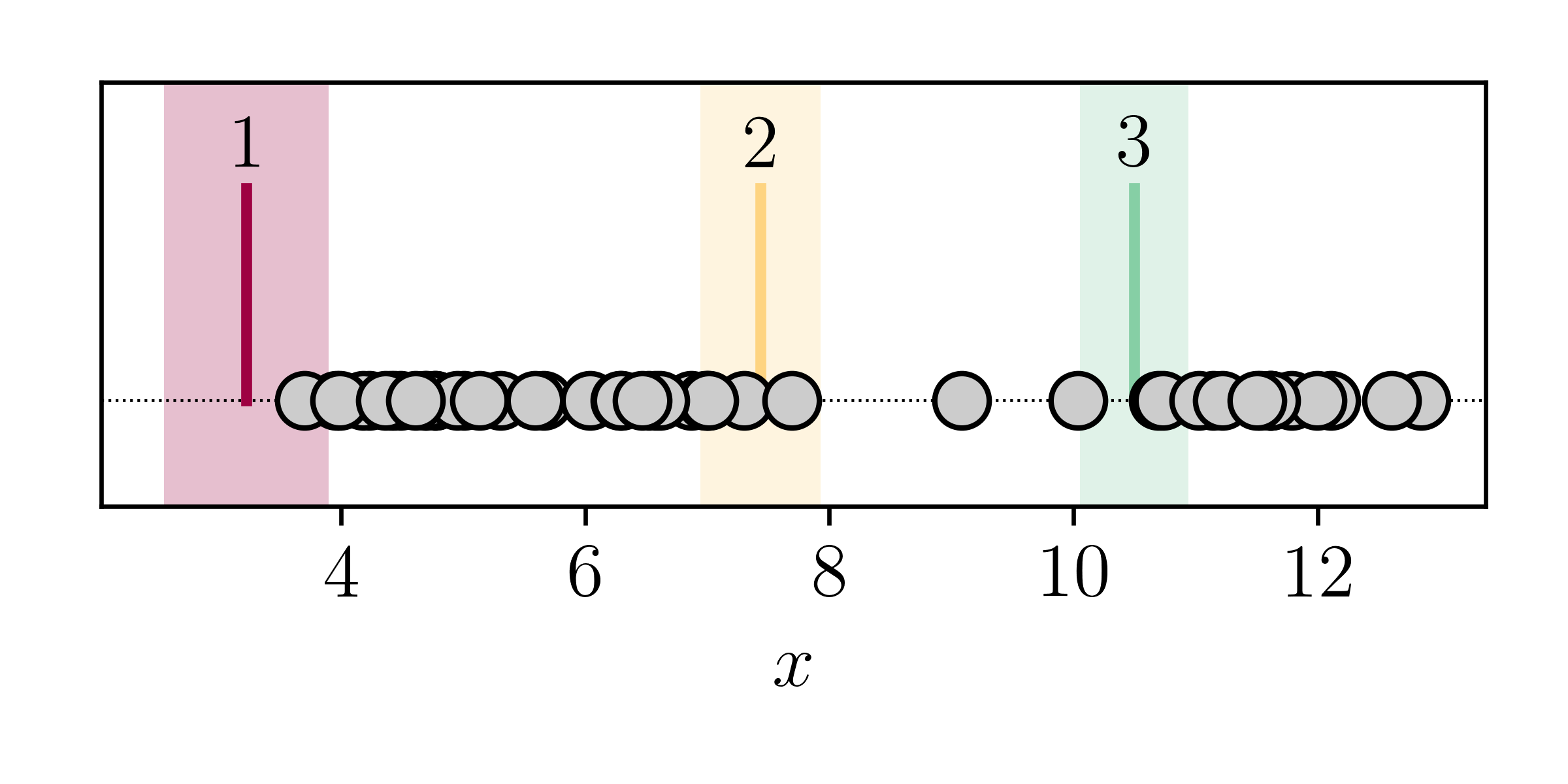
Even though these initial guesses are bad, we can still estimate the probability of each data point being drawn from each component. For example, the points near our random guess of the red line are probably best described by the first component, and those near the yellow line are probably best described by the second component, and so on.
How do we formalise this? What we want is the posterior probability of membership for belonging to one component, compared to all components. In other words, we want the probability of belonging to the \(k\)-th component given the data \(x_i\)
\[
p(\mathcal{M}_k|x_i) = \frac{p(x_i|\mathcal{M}_k)p(\mathcal{M}_k)}{\sum_{j=1}^{K}p(x_i|\mathcal{M}_j)p(\mathcal{M}_j)}
\]
where we often assume priors for individual components \(p(\mathcal{M}_k)\) to be equal. If we calculate these membership probabilities for all data points, given our random estimates of the initial means and variances, we find:
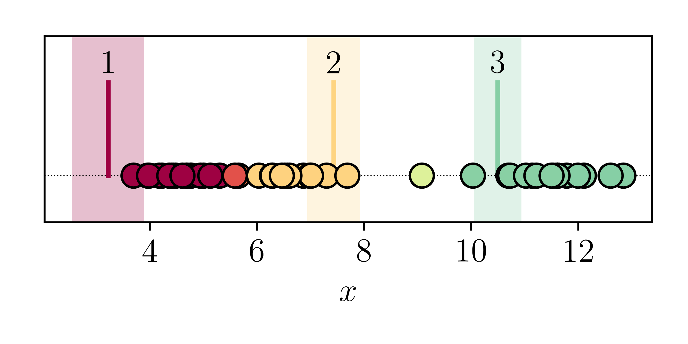
Where it is clear that data points near the mean are coloured by the component colour. But data points in between two components have a membership proportion that is split between the two components. For those data points we don't know which component they are best described by!
A chicken and egg problem
Hopefully you can appreciate that we have a kind of chicken and egg problem here:
- We need the component parameters to be able to estimate the source component for each data point!
- We need to know the source component for each data point to estimate the component parameters!
The Expectation-Maximization algorithm is simply where we alternate between these two steps. First we start with some randomly chosen initial parameters, and then we:
- Calculate our expectation for which data point is drawn from what component, conditioned on our estimate of the model parameters.
- Update our estimates of the model parameters, conditioned on the partial assignments (or propotions) we have calculated for each data point to belong to what component.
Expectation-Maximization is mathematically guaranteed to increase the log-likelihood with every step!
There's no need for us to take derivatives and work out the optimal path forward. There are no false turns! There are no optimisation hyperparameters for us to tune! All we need to do is step between expectation, maximization, expectation, maximization, ..., and with every Expectation-Maximization step we are guaranteed to increase the log likelihood! And because the log likelihood is improving it means with every step our estimate of the model parameters is improving! Hopefully now you can understand why the Expectation-Maximization algorithm is so important for data analysis and machine learning.
Here you can see this working in practice. We start with totally random guesses of the model parameters, and run Expectation-Maximization for 100 steps.
You can see that it doesn't take long for the algorithm to settle in to a minima, and then with each update there is only a very small change to the model parameters. Notice the "jittery"-ness, where the algorithm is stepping between calculating the expectation of individual data points, and then maximizing the log likelihood by updating the model parameters.
Implementation
Let us consider a Gaussian mixture model where there are \(N\) data points each of \(D\) dimensions. We will assume that the data are drawn from a mixutre of \(K\) Gaussian components such that: \[ p(y|\theta) = \sum_{k=1}^{K} w_{k}p_k(y|z_k,\theta_k) \] where \(\sum^K w_k = 1\) and \(\theta_k = \{\mu_k, \Sigma_k\}\).
In the expectation step we want to compute the membership probabilities, given the current estimate of the model parameters. That is to say that we want to create a \(N\) by \(K\) matrix where for each row (data point) the probabilities sum to 1, and for each column (mixture) the weights sum to the effective number of data points described by that component. To calculate \(w_{nk}\), \[ w_{nk} = p(z_{nk} = 1|y_n,\theta) = \frac{w_kp_k(y_n|z_k,\theta_k)}{\sum_{m=1}^{K}w_mp_m(y_n|z_m,\theta_m)} \] where \[ p_k(\vec{y}|\vec{\theta}_k) = \frac{1}{(2\pi)^{D/2}|\Sigma_k|^{1/2}}\exp\left[-\frac{1}{2}\left(\vec{y}-\vec{\mu}_k\right)\transpose\vec{\Sigma}_k^{-1}\left(\vec{y}-\vec{\mu}_k\right)\right] \]
In the maximization step we want to compute the model parameters, given the current estimate of the membership probabilities. Given an \(N\) by \(K\) matrix of membership responsibilities, \[ N_k = \sum^{N}w_{nk} \] describes the effective number of data points described by the \(k\)-th mixture, and \(\sum^{K}w_{nk} = 1\) for every data point. Then the new estimates of the weights are: \[ w_k^{\mathrm{(new)}} = \frac{N_k}{N} \] And the means can be updated: \[ \mu_k^{\mathrm{(new)}} = \frac{1}{N_k}\sum_{n=1}^{N} w_{nk}\vec{y}_n \] And then the covariance matrices: \[ \vec{\Sigma}_k^\mathrm{(new)} = \frac{1}{N_k}\sum_{n=1}^{N}w_{nk}\left(\vec{y}_n-\vec{\mu}_k^\mathrm{(new)}\right)\left(\vec{y}_n-\vec{\mu}_k^\mathrm{(new)}\right)\transpose \]
Caveats
Expectation-Maximization algorithm still has it's caveats. Your problem will still be non-convex: an algorithm won't solve that. That means that initialisation will still be important, and you will have local minima. There will still be identifiability problems too, unless you have some joint priors to enforce an ordering or labelling of the components. And you still won't know how many components you should have!
We usually continue Expectation-Maximization until the change in the log likelihood is very small, just like a convergence threshold for an optimisation algorithm, or up until some maximum number of iterations.
Summary
The Expectation-Maximization algorithm is extremely simple to implement and is one of the most important algorithms in data analysis and machine learning. It appears in classification, regression, clustering, and many other topics. We will explore some of these in the next week as we introduce some basic topics on supervised machine learning.