(This lecture has a lot of linear algebra in it, even though I have omitted the proofs! Sometimes there's so much math that MathJax fails to render the LaTeX correctly. If that happens to you, just refresh until things work properly.)
In the last class we used the odds ratio
Gaussian processes sit at a very important intersection between data analysis and machine learning: they are very popular in both "fields" because they are extremely flexible, (somewhat) interpretable, and probabilistic! So you should learn about them!
An important preface
There are several ways to think of Gaussian processes. And there are many ways that Gaussian processes will relate to other concepts that you have covered before, including those from basic signal processing, probabilities, and quantum mechanics, to name a few. You will probably find that some parts of Gaussian processes are easy to understand, and some parts are extremely difficult to understand. For this reason I am going to explain Gaussian processes in two different ways. I encourage you to accept that there will be one way that is easier for you to understand than the alternative. And for the purposes of being time-limited, I encourage you to be mentally prepared to accept something to be true without going through the rigorous linear algebra proof!
The two views of Gaussian processes that we will discuss in this class will be the weight-space view and the function-space view. We will introduce the weight-space view first because it has more mathematical rigour, and then we'll introduce the function-space view to help you conceptualise this crazy idea!
In both views the end result will be the same. Instead of modelling the data in data space, a Gaussian process models the correlation between data points based on the distance between those points. In other words, the covariance matrix describes the data rather than a prescribed model \(f(x)\).
\[ \newcommand\vectheta{\boldsymbol{\theta}} \newcommand\vecdata{\mathbf{y}} \newcommand\model{\boldsymbol{\mathcal{M}}} \newcommand\vecx{\boldsymbol{x}} \newcommand{\transpose}{^{\scriptscriptstyle \top}} \renewcommand{\vec}[1]{\boldsymbol{#1}} \newcommand{\cov}{\mathbf{C}} \]Weight-space view
Let us imagine that we have some data that are Gaussian-distributed such that the log probability is
\[
\log p(\vecdata|\vectheta,\vec{\sigma}_y,\vec{x}) = -\frac{1}{2}\left(\vecdata - \vec{\mu}(\vectheta)\right)\transpose\cov^{-1}(\vecdata - \vec{\mu}(\vectheta)) -\frac{1}{2}\log{|2\pi\cov|} \quad .
\]
We will assume that \(\vecdata\) is a one-dimensional vector of \(N\) data points and \(\vec{\mu}(\vectheta)\) describes the mean model given some parameters \(\vectheta\). We will also assume that there are a number of systematic effects that we can't explicitly write down functions for, but we know that those systematic effects are present in the data. An example could be that if your data are some time series observations of the brightness of a star measured from a satellite in space
Because we don't know the importance of each systematic, we will introduce each systematic to have an assigned weight \(w\). For brevity we will use \(\vec{\psi} \equiv \{\vec{\sigma}_y,\vec{x},\vec{A}\}\). We should then re-write our log probability to be
\[
\log p(\vecdata|\vectheta,\vec{\psi},\vec{w}) = -\frac{1}{2}\left(\vecdata - \vec{\mu}(\vectheta) - \vec{A}\vec{w}\right)\transpose\cov^{-1}(\vecdata - \vec{\mu}(\vectheta)- \vec{A}\vec{w}) -\frac{1}{2}\log{|2\pi\cov|} \quad .
\]
where \(\vec{w}\) is a \(M\)-dimensional vector of unknown weights, and \(\vec{A}\) is an \(N \times M\) dimensional matrix of possible systematic effects, which we will define as the design matrix. And the design matrix \(\vec{A}\) could include any number of things, including telescope temperature \(T\), or temperature squared \(T^2\), or the number of pieces of toast I had for breakfast each day while the telescope observed the star.
In practice we don't really want to know the weights. We just want to marginalise over them! You will recall though, that in order to marginalise over some parameter, we must introduce a prior on that parameter. We will assume a multivariate Gaussian prior on the weights that is centered at zero \[ p(\vec{w}) \sim \mathcal{N}\left(\vec{0},\vec{\Lambda}\right) \] with some covariance matrix \(\vec{\Lambda}\) such that \[ \log{p(\vec{w})} = -\frac{1}{2}\vec{w}\transpose\vec{\Lambda}^{-1}\vec{w} - \frac{1}{2}\log{|2\pi\vec{\Lambda}|} \quad . \]
Using the rule of conditional probability we can marginalise out \(\vec{w}\)
\[
p(\vec{y}|\vec{\theta},\vec{\psi}) = \int_{-\infty}^{+\infty} p(\vec{w})p(\vec{y}|\vectheta,\vec{\psi},\vec{w}) d\vec{w}
\]
which expands to become something nasty looking:
\[
p(\vec{y}|\vec{\theta},\vec{\psi}) = \int_{-\infty}^{+\infty} \frac{1}{|2\pi\vec{\Lambda}|^\frac{1}{2}} \exp{\left(-\frac{1}{2}\vec{w}\transpose\vec{\Lambda}^{-1}\vec{w}\right)\frac{1}{|2\pi\cov|^\frac{1}{2}}} \exp{\left(-\frac{1}{2}\left[\vec{r}-\vec{A}\vec{w}\right]\transpose{}\cov^{-1}\left[\vec{r}-\vec{A}\vec{w}\right]\right)} d\vec{w}
\]
where things look a bit nicer if we take \(\vec{r} = \vec{y} - \vec{\mu}(\vectheta) \) and write
\[
p(\vec{y}|\vec{\theta},\vec{\psi}) = \frac{1}{|2\pi\vec{\Lambda}|^\frac{1}{2}|2\pi\cov|^\frac{1}{2}} \int_{-\infty}^{+\infty} \exp\left(-\frac{1}{2}\vec{z}\right) d\vec{w}
\]
where
\[
\vec{z} = \vec{w}\transpose\vec{\Lambda}^{-1}\vec{w} + (\vec{r} - \vec{Aw})\transpose\cov^{-1}(\vec{r}-\vec{Aw}) \quad .
\]
Since this integral is over \(d\vec{w}\) and we know the magical properties of Gaussians,
It is worthwhile stopping for a moment to consider what we have done. We have introduced a design matrix \(\vec{A}\), which could include any number of \(M\) potential features (e.g., spacecraft temperature). Importantly, the design matrix could include features like \(\vec{x}\), \(\vec{x}^2\), ..., and any number of other basis functions. This still remains a linear problem (even if the design matrix contains non-linear terms of \(\vec{x}\)) because the design matrix is only calculated once. If we were to include \(M\) features that are all increasing terms of \(\vec{x}\) to some power, you can see that the weights \(\vec{w}\) that we have marginalised over are actually the coefficients of those \(\vec{x}^m\) terms. For example if the design matrix contained the entries \[ \vec{A}\transpose = [\vec{1}, \vec{x}, \vec{x}^2, \vec{x}^3, \vec{x}^4, \vec{x}^5, \cdots] \] then the dot product \(\vec{Aw}\) expands to \[ w_0 + w_1\vec{x} + w_2\vec{x}^2 + w_3\vec{x}^3 + w_4\vec{x}^4 + w_5\vec{x}^5 + \cdots \] which you will recognise as a polynomial problem, yet it remains a linear problem because \(\vec{A}\) is just an array that is calculated once and never changes.
You may be thinking: what about \(\vec{\Lambda}\)? Or why did we introduce \(\vec{\Lambda}\) and why does it not appear with \(\vec{\theta},\vec{\psi}\) since the probability of \(\vec{y}\) is actually conditioned on \(\vec{\Lambda}\). We're about to explain why, and things are going to get funky.
The kernel trick
We get to arbitrarily set the number of \(M\) features that we will put into our design matrix \(\vec{A}\). What happens as \(M \rightarrow \infty\)? The shape of \(\vec{A}\) is \(N \times M\) and the size of \(\vec{\Lambda}\) is \(M \times M\), so we will have some infinitely large matrices to take inner products of. But what would be in our infinite set of features, and why would we want to create infinitely large matrices?
It turns out this isn't such a crazy idea, for two reasons. The first reason relates to the complexity of the data. Imagine if the data has some highly non-linear relationship. If your design matrix only included linear terms (e.g., like \(\vec{x}\)) then your model won't be able to capture those non-linear relationships. And because we are thinking about the Gaussian process in the context of modelling unknown (potentially non-linear) systematics, we do want to capture those relationships! But if we included an infinite number of possible features (e.g., either \(\vec{x}^m\) terms or better yet \(\sin(\vec{x})\) and \(\cos(\vec{x})\) terms) then the model will be able to capture all kinds of non-linearities in the data. That is to say: even if there is no linear relation in the data space, there may be linear relations in a higher dimensional feature space
The second reason relates to a special property of \(\vec{A}\vec{\Lambda}\vec{A}\transpose\). You will notice that this term contains only inner products. It turns out if you have an infinite dimensional set of vectors that only contain inner products, then you don't need to explicitly build these matrices or take their inner products! Instead you can re-cast the problem as a function where the element-wise entries of the matrix of \(\vec{A}\vec{\Lambda}\vec{A}\transpose\) can be computed directly
\[
\left[\vec{A}\vec{\Lambda}\vec{A}\transpose\right]_{nn'} \rightarrow k(\vec{x}_n,\vec{x}_{n'})
\]
without needing to explicitly construct those infinite dimensional matrices! As long as the output of the element-wise evaluations of that function (which we call the kernel function) produces a positive semi-definite matrix,
What this means is that we can implicitly include a \(N \times \infty\) shaped design matrix \(\vec{A}\) of features without ever having to construct it or without ever computing the inner product \(\vec{A}\vec{\Lambda}\vec{A}\transpose\)! It also means that we can ignore the dependence on \(\vec{\Lambda}\) (and \(\vec{A}\)) because we will re-write our problem as a function \(k(\vec{x}_{n},\vec{x}_{n'})\) instead of an inner product of infinite dimensional matrices.
Before we introduce the function-space view it may be useful to see how predictions are actually made. Let us define the kernel function as \(k(\vec{x},\vec{x}')\) and after computing the element-wise entries you can construct a covariance matrix \(\vec{K}\). Now let us re-cast our probability \(p(\vec{y}|\vec{\theta},\vec{\psi})\) as \[ p(\vec{y}|\vec{\theta},\vec{\psi}) = \frac{1}{|2\pi(\cov + \vec{K})|^\frac{1}{2}}\exp\left(-\frac{1}{2}(\left[\vec{y} - \vec{\mu}(\vec{\theta})\right]\transpose\left[\cov + \vec{K}\right]^{-1}\left[\vec{y}-\vec{\mu}(\vec{\theta})\right]\right) \quad . \] We will denote \(\vec{y_*}\) as the \(y\)-value(s) we want to predict at given \(\vec{x_*}\) locations. To clarify: \(\vec{x}\) and \(\vec{y}\) will represent observations, and \(\vec{y_*}\) are the predictions we want to make for the values of \(y\) at \(x\)-positions \(\vec{x_*}\). We would like to make predictions for these values \(\vec{y_*}\). That is we want to compute the probability of \(\vec{y_*}\) given \(\vec{x_*}\) and the existing set of observations \(\{\vec{x},\vec{y},\vec{\sigma_y}\}\), \[ p(\vec{y_*}|\vec{x_*}, \vec{y}, \vec{x}, \vec{\sigma_y}, \vec{\theta}) = \mathcal{N}\left(\vec{y_*}|\vec{\mu_*},\vec{V_*}\right) \] where it can be shown that \[ \begin{eqnarray} \vec{\mu_*} &=& \vec{K_*}\cov^{-1}\vec{y} \\ \vec{V_*} &=& \vec{K_{**}} - \vec{K_*}\cov^{-1}\vec{K_*}\transpose \end{eqnarray} \] where \(\vec{K_{**}}\) is the constructed covariance matrix for just the \(\vec{x_*}\) points, and \(\vec{K_*}\) is the constructed covariance matrix for the observed points and the new points. You can think of this as \(\vec{K_{**}}\) being the Gaussian process prior for the variance in the limit of having no observations, and the \(\vec{K_*}\cov^{-1}\vec{K_*}\transpose\) incorporates the observations (and their uncertainties) and the correlation between the observed and new data points.
Before we dive deep into how we construct the covariance matrices \(\vec{K}\), or even what set of kernel functions \(k(\vec{x},\vec{x}')\) are allowed, let's introduce the function-space view.
Function-space view
A Gaussian process is a collection of random variables, any finite number of which have a joint Gaussian distribution.
Let us imagine that there are two axes \(x\) and \(y\). We know that we will collect some data of \(x\) and \(y\), but before we measure any data there are literally an infinite number of functions that could generate data from \(x\) to \(y\). It could be a straight line, or a polynomial with an infinite number of terms! Before taking any data we have no idea what the true function is.
Gaussian processes assign a prior probability to each of the infinite number of possible functions. When we measure some data, the predictions we make for other locations (in \(x\) and \(y\)) are conditioned on the observations that we have seen. The more data we observe, the more confident we become in the predictions elsewhere. Consider this excellent example below from Distill
Here you can see that when we start off with no data there is some variance in \(y\) (that we have set) and the mean of the model is \(y = 0\). But as soon as we add a (noiseless) data point, the Gaussian process is forced (by definition) to go through that data point. And our predictions for nearby values has suddenly changed because our predictions are conditioned on the data set
Let me write that again. A Gaussian process assigns a prior probability to each of the infinite number of possible functions. The observations restrict the set of possible functions!
We are used to thinking about data being one dimensional in the \(x\)-direction and one dimensional in the \(y\)-direction. Instead, let us imagine that the \(y\) data points are drawn from one huge multivariate Gaussian distribution, where the dimensionality of the Gaussian is the same as the number of \(y\) data points you have. Then imagine that there is some covariance between those dimensions (those \(y\) data points) such that the value of one data point \(y_2\) depends on the value of other data points (i.e., \(y_1\)) and it depends on how far away \(x_1\) and \(x_2\) are. In a sense, nearby data points could be more correlated than distant points. If you described your covariance matrix in the right way, the covariance matrix (and a mean function) can fully describe your data without having to have an explicit functional form between \(x\) and \(y\) — because the Gaussian processs already includes all infinite number of possible functional forms!
Consider this below for just two data points \(x_1\) and \(x_2\):
With a correctly defined covariance matrix you can predict the expectation value and variance of \(x_2\) given some observation \(x_1\). It's a little counter-intuitive to think about how the covariance matrix should look for various trivial problems (e.g., a straight line) but we will get there!
Kernels
We have shown that some data set can be described by the structure in the covariance matrix rather than an explicit functional relationship. But we have not described what kernel functions are available — only that they must construct a covariance matrix \(\vec{K}\). In general your kernel function only needs to produce a non-negative semi-definite covariance matrix, but in practice there are a few kernels that are used (or combined) for different problems.
Kernels are broadly described as either being stationary or non-stationary. Stationary kernels are functions that depend only on the radial distance between points in distance space, and non-stationary kernels are those that depend on the value of an input coordinate (e.g., to model an effect at a specific location in \(\vec{x}\)).
You will see that each kernel has parameters (or rather: hyperparameters) associated with them. We call them hyperparameters because they do not directly describe the data. Instead they describe the structure of the covariance matrix that describes the data. These hyperparameters control things like the magnitude of the variance, and the scale length over which points no longer become correlated. For periodic kernels, a periodic hyperparameter is obviously required. These hyperparameters become unknown variables of your model (like \(\vec{\theta}\)) that you can either optimise, or sample from. But you can see that just a few hyperparameters gives you a lot of model flexibility!
If you hadn't already thought about it, you should realise that even though the weight-space view showed us that we were incorporating a design matrix of infinite dimensions, one Gaussian process kernel function will not give infinite flexibility. For example, a stationary kernel has behaviour at a fixed location, and similarly a periodic kernel is explicitly necessary if you want to allow periodicity in the underlying systematic effects you are modelling. Thankfully, kernels can be added or multiplied to produce different effects.
An example: atmospheric carbon dioxide
Atmospheric CO2 levels is a common example used to show the combination of Gaussian process kernels to describe non-linear data.george package. Here we will exactly follow the example from the george documentation on Hyperparameter optimization.
First let's plot the data.
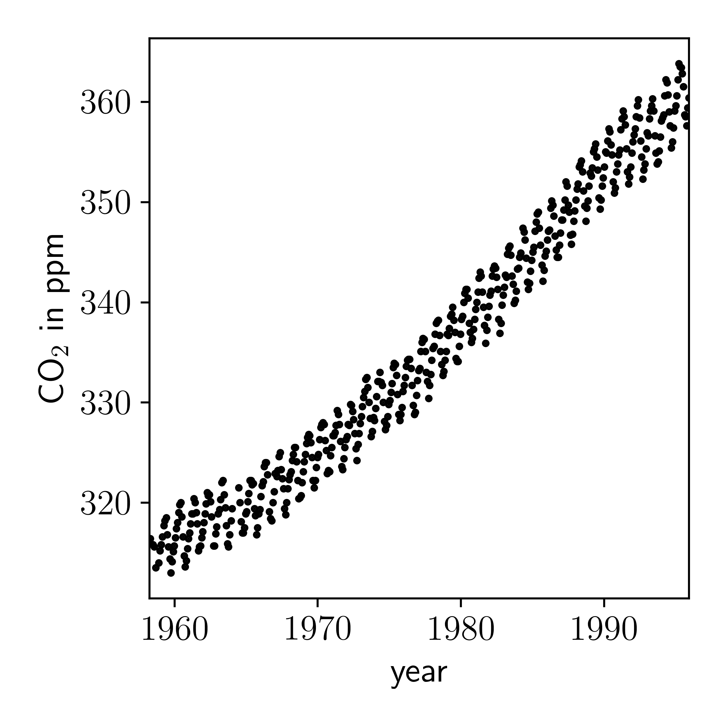
It is clear that there is a quasi-periodic signal here that is increasing with time. Instead of trying to find some functional relationship between time and CO2 level, following other examples
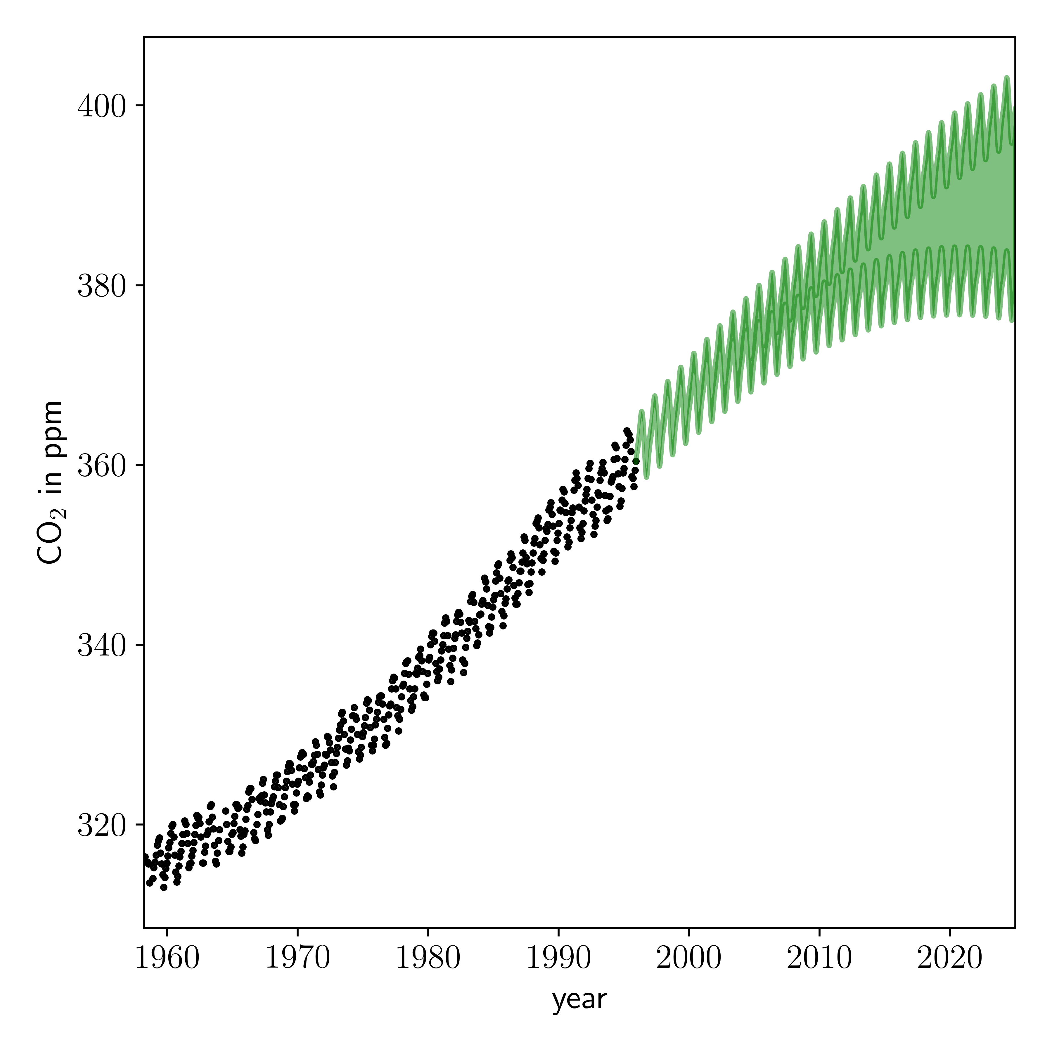
Continuing to follow the george example, which is replicated here in parts, we will construct the kernels and optimise the hyperparameters from the result in Rasmussen & Williams:
Now we will use the Gaussian process to make predictions for future observations, conditioned on what we have already observed, and conditioned on our optimised value for the hyperparameters:
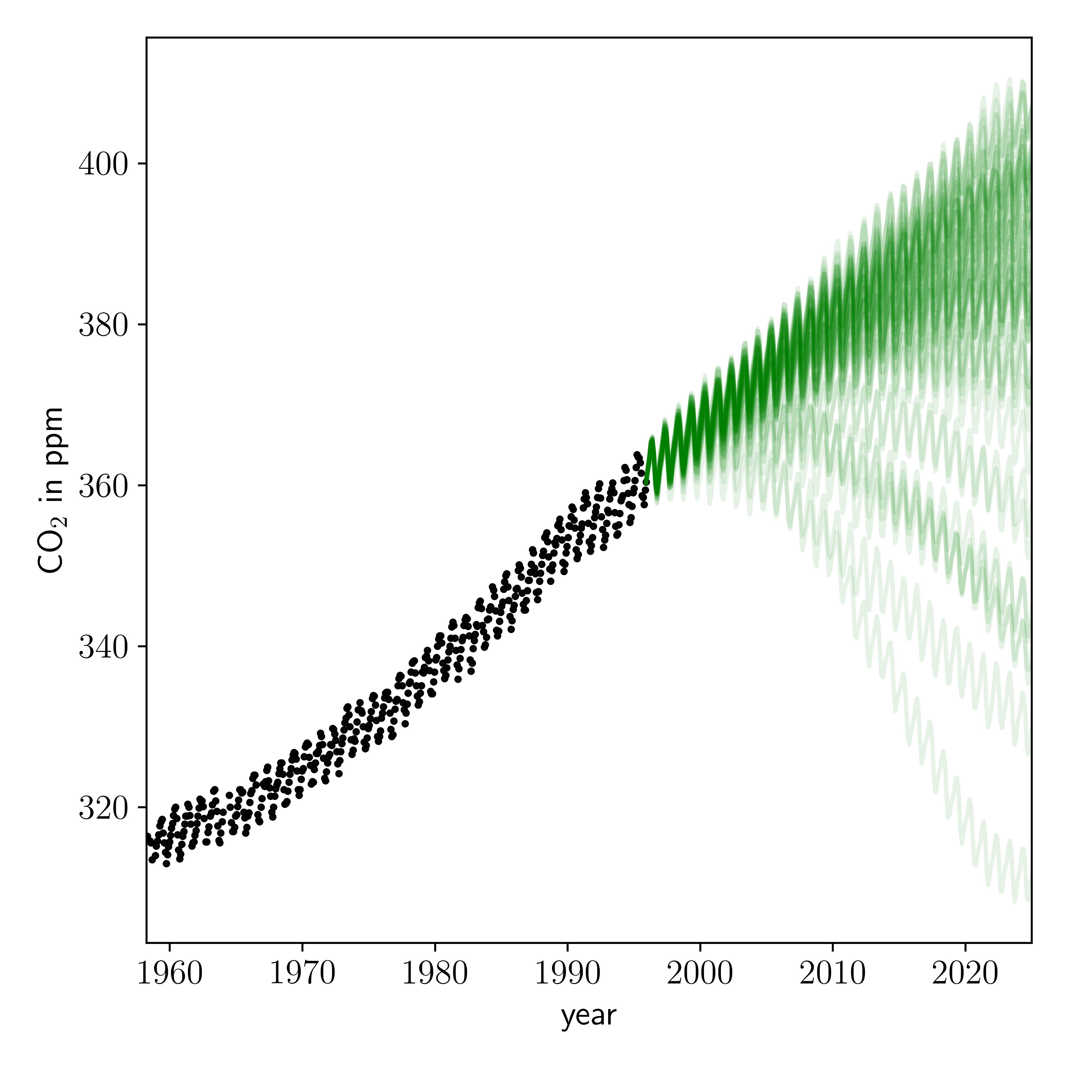
Looks pretty good to me! But these predictions are conditioned on our point estimate of the kernel hyperparameters. We actually want to sample those parameters and make predictions based on the posterior distribution of those parameters.
Well the predictions look sensible, albeit mostly depressing.
Summary
A Gaussian process assigns a prior probability to each of an infinite number of possible functions. Every observation restricts the set of possible functions. Gaussian processes have important applications in machine learning and data analysis more broadly, because they are both probabilistic (e.g., they preserve uncertainty), somewhat interpretable, and extremely flexible!
In the next class we are going to continue on advanced modelling techniques and introduce you to the concept of hierarchical models, and probabilistic graphical models.