In the next hour
- learn (or be reminded of) what Markov chain Monte Carlo (MCMC) is;
- learn (or be reminded of) how some variations of MCMC exist, including:
- the Metropolis method;
- affine-invariant methods like the
emceeimplementation; - Hamiltonian methods.
- learn (or be reminded of) how to tune MCMC samplers;
- learn (or be reminded of) how to diagnose outputs from MCMC samplers;
- implement your own Metropolis MCMC sampler; and
- implement your own Hamiltonian Monte Carlo sampler.
What is MCMC and why would we use it?
Markov chain Monte Carlo (MCMC) methods are for approximating integrals.
MCMC methods are used to draw samples from a continuous random variable, where the probability density for each sample will be proportional to some known function. In most cases that you (the physicist) will use MCMC, the continuous random variable you are drawing from is the posterior probability, and the integral that you are approximating is the posterior probability density function (pdf; the area under the curve of posterior probability).
The Markov chain part of the name is a stochastic process that describes a sequence of events, where each event depends only on the outcome of the immediately previous event. You can think of it as walking, where after each step you roll a four-sided die to decide where to move next: north, east, south, or west. Because each roll of the dice is independent, your current position only depends on your last position, and the roll of the dice.
The Monte Carlo part of the name describes randomness. Let's say that we roll the die as before, but before taking a step we look in that direction and then decide if we actually want to step there or not. For theatrical purposes we will say that there are dropbears scattered around you, and dropbears are known to chase humans who have walking patterns that don't follow a Markov chain Monte Carlo method.
That's (almost) a Markov chain Monte Carlo algorithm. Except for the dropbears
There are many variations of MCMC available, and many are tailored for particular problems (e.g., multi-modal problems). All of them share two properties:
- how to decide on the new proposed step in parameter space, and
- how to decide on whether to accept or reject that proposal.
You can't do this ad hoc. There are Rules™. If your answers to (1) and (2) above don't follow the Rules™ then you lose all guarantees for your sampler to accurately approximate the integral. The first Rule™ is that of detailed balance: it must be equally likely to move from point \(A\) in parameter space to point \(B\), as it is to move from point \(B\) to point \(A\). In other words, the probability of movement must be just as reversible. Your method for proposing a new step in parameter space must follow this Rule™, or it must correct for detailed balance in the accept/reject step. You can't easily do the correction causally, either: you must be able to prove that the correction is (well,..) correct from a mathematical perspective. You must also be able to show that the proposal distribution \(q(\theta'|\theta_k)\) is properly normalised: the integration over \(\theta'\) should equal unity. Lastly, you must make the proposals in the same coordinates which your priors are specified. Otherwise you must add a Jacobian evaluation to the log probability in order to account for the change of variables.
The Metropolis algorithm
The Metropolis algorithm
With the current position \(\theta_k\) and the proposal distribution \(q(\theta'|\theta_k)\) the algorithm is as follows:
- Propose a position \(\theta'\) by drawing from the proposal distribution \(q(\theta'|\theta_k)\).
- Compare the proposed position with the current position by calculating the acceptance ratio \(\alpha = f(\theta')/f(\theta_k)\).
- Draw a random number \(u \sim \mathcal{U}\left(0, 1\right)\):
- If \(u \leq \alpha\) then we accept the proposed position and set \(\theta_{k+1} = \theta'\).
- If \(u > \alpha\) then we reject the proposal and keep the existing one by setting \(\theta_{k+1} = \theta_{k}\).
Let's implement this in code. First we will generate some faux data where we know the true value, which is essential for model checking! We will adopt the following model
\[
y \sim \mathcal{N}\left(\mu, \sigma\right)
\]
where the data \(y\) are drawn from a Gaussian distribution centered on \(\mu\) with standard deviation \(\sigma\), but the data \(y\) also have some uncertainty of \(\sigma_y\). The unknown model parameters are those of the Gaussian: \(\theta = \{\mu, \sigma\}\).
Now let's define our log prior, log likelihood, and log probability functions:
And we're ready to implement the Metropolis MCMC algorithm:
The astute among you will see that we made some decisions without explicitly talking about them. One of those is the number of iterations: 10,000. Because we have a Markov chain, the position of each step depends on the previous step. But in the end what we want are independent samples of the posterior density function. How can we have an independent sample if each position depends directly on the last position? And how can the sampling be independent if we decided on the initialisation point? We will discuss this in more detail below, but the short answer is that you need to run MCMC for a long time.
But how long is the burn-in? This relates to the Markov property (and many other things). Each sample is dependent on the previous sample. But the 100th sample depends very little (or at all) on the 1st sample. That means the chain has some auto-correlation length where nearby samples are correlated with each other. If you have a long correlation length then it means you don't have many effective independent samples of the posterior pdf because your samples are correlated with each other. If you have short correlation lengths then you will have many effective independent samples (for the same length chain). Samplers that produce shorter auto-correlation lengths for the same number of objective function evaluations are more efficient. We discuss this in more detail below.
The other decision we made without discussing it relates to the proposal distribution \(q(\theta'|\theta_k)\). We explicitly stated that we would adopt a Gaussian distribution centered on the point \(\theta_k\), but we made no mention of the covariance matrix for that proposal distribution. In the code we have adopted an identity matrix
\[
\mathbf{I} = \begin{bmatrix} 1 & 0 \\ 0 & 1 \end{bmatrix}
\]
which effectively defines the scale of the proposal step in each direction. We get to choose this step size, and it can be different for each parameter!
Let's plot the value of the model parameters at each iteration.
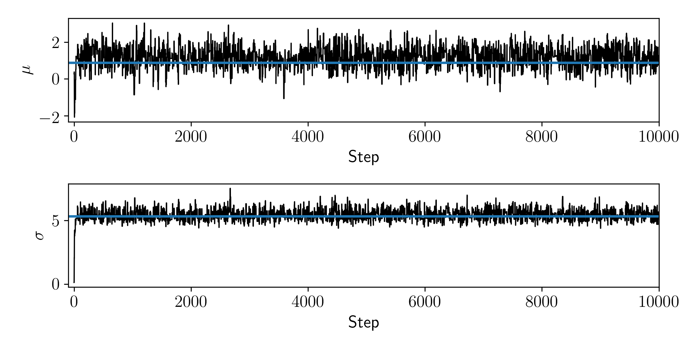
You can see that the walker quickly moves from the initial position and settles around the true values shown in blue. That looks sensible. For now we will not investigate any diagnostics, and simply say that is good enough because we don't intend to use these samples for any proper (scientific) inference.
Affine-invariant methods
There are many MCMC samplers but there is barely time in this class to introduce three. The second is the affine-invariant MCMC sampleremcee Python package.
Affine-invariant methods use multiple walkers (chains) to propose a new position. At each step the walkers will draw a line between another randomly chosen walker and a new proposal is generated somewhere along that line. This reduces the number of hyperparameters (e.g., like those along the diagonal of the proposal distribution) to just 1 or 2. This implementation is what makes sampling correlated parameters so efficient, because the proposals can be drawn along some line between walkers. The proposal itself does not follow detailed balance since there is a preferred direction for proposals to be made. However, the correction to this proposal is done in the accept/reject step. The growth of the walkers is controlled by \(\alpha\), a stretch parameter that controls how quickly the walkers will expand into the typical set. It's called a stretch parameter because it's easy for parameters to stretch out, but harder for them to collapse back in. That means it's a good idea to initialise your walkers in a very small ball in parameter space (e.g. at the optimised point) and watch them stretch out in parameter space.
Affine invariant samplers are excellent if you have relatively low numbers of model parameters, and you don't have gradient information for your log probability function. Affine invariant samplers are not suitable for high dimensional problems, and can fail quietly.
Hamiltonian Monte Carlo
In the optimisation class we emphasised
The answer is an overwhelming yes, but the sampler must still obey detailed balance. The way we will do this is by introducing new variables that will help guide the proposal distribution along the curvature of the objective function, but make sure that the target distribution (the posterior) remains independent of the variables we have introduced.
You will recall that a Hamiltonian uniquely defines the evolution of a system with time. Specifically, Hamiltonian dynamics describes how potential energy is converted to kinetic energy (and vice versa). At time \(t\), a particle in some system has a location \(\vec{x}\) and momentum \(\vec{p}\), and the total energy of the system is given by the Hamiltonian
\[
\mathcal{H}\left(\vec{x}, \vec{p}\right) = U(\vec{x}) + K(\vec{p})
\]
which remains constant with time. Here we follow the usual nomenclature where \(U(\vec{x})\) describes the potential energy and \(K(\vec{p})\) is the kinetic energy. The location \(\vec{x}\) is our location in the parameter space, which we previously called \(\vec{\theta}\), \(\vec{\theta} \equiv \vec{x}\). We will introduce the momentum vector \(\vec{p}\) as auxilary (nuisance) variables, which we have yet to define. The momentum vector \(\vec{p}\) has the same dimensionality as \(\vec{x}\), so we are immediately duplicating the number of parameters in the problem!
The time evolution of the system is described by the set of differential equations \[ \frac{d\vec{x}}{dt} = +\frac{\partial\mathcal{H}}{\partial\vec{p}} \quad \textrm{and} \quad \frac{d\vec{p}}{dt} = -\frac{\partial\mathcal{H}}{\partial\vec{x}} \quad . \] We want to develop a Hamiltonian function \(\mathcal{H}(\vec{x},\vec{p})\) that will let us efficiently explore the target distribution \(p(\vec{x})\).
Imagine if a particle were moving through parameter space and its movement followed a Hamiltonian. If the target density were a two dimensional Gaussian with an identity matrix as the covariance matrix, then a particle moving through this density (with constant energy) would be akin to a particle moving in a circular motion around the center of the Gaussian. In other words, it would be like the particle is orbiting around the Gaussian. But we don't want the particle to just explore one slice (or one line of constant energy) in the parameter space: we want the particle to explore all of parameter space. For this reason, we need to consider particles to have a distribution of energies where the particles with that distribution of energies would efficiently sample the target density.
For reasons outside the scope of this class, we will use the canonical distribution. With an energy function \(E(\vec{\theta})\) with some set of parameters \(\vec{\theta}\), the canonical distribution is
\[
p(\vec{\theta}) = \frac{1}{Z}\exp\left[-E\left(\vec{\theta}\right)\right]
\]
where \(Z\) is a normalising constant
We have defined our Hamiltonian. But how will we use it in practice?
- Draw from the momentum distribution \(p(\vec{p})\) to set the momentum \(p(\vec{p}_k)\) for the current position \(\vec{x}_k\): \(\vec{p}_k \sim \mathcal{N}\left(\vec{0}, \vec{I}\right)\).
- Given the current position \(\vec{x}_k\) and momentum \(\vec{p}_k\), integrate the motion of the fictitious particle for \(L\) steps with a step-size of \(\delta\) (which we have yet to define), requiring that the total energy of the Hamiltonian remains constant. The position and momentum of the particle at the end of the integration are \(\vec{x}'\) and \(\vec{p}'\), respectively.
- If we always integrated forward in time then it would not maintain detailed balance. To correct for this we flip the momentum vector of the particle at the end of integration so that it becomes \(-\vec{p}'\). This alternates the direction of the particle at each step, equivalent to integrating forward in time and then backward et cetera.
- Calculate an acceptance ratio \(\alpha\) for the proposed position and momentum \((\vec{x}',-\vec{p}')\)compared to the initial position and momentum vector \((\vec{x}_k,\vec{p}_k)\)
Just like Metropolis! \[ \alpha = \exp\left[-U(\vec{x}') + U(\vec{x}_k) - K(-\vec{p}') + K(\vec{p}_k)\right] \] - Draw a random number \(u \sim \mathcal{U}\left(0, 1\right)\)
- If \(\alpha >= u\), accept the proposed state and set \(\vec{x}_{k+1} = \vec{x}'\).
- If \(\alpha < u\), reject the proposed state and set \(\vec{x}_{k+1} = \vec{x}_k\)
If our integrator was well behaved then we would almost always end up accepting the proposed distribution. That's because we are drawing from a symmetric momentum distribution that helps guide the particle along some constant energy, and is independent of the position vector. The main reason why we wouldn't accept a proposal would be because we are using a numerical integrator (not an exact integration), and the final position of the particle will not always exactly maintain constant energy.
Since constant energy is so important to us, when integrating the motion of the particle you should use a symplectic integrator. Specifically, the leapfrog integration scheme is well-suited to this problem because the position and momentum vectors are independent of each other.
Tuning
Create a new file and run the example code for the Metropolis MCMC sampler above. First make sure that you get the same results as shown in the figure. Once you're satisfied with that, copy the file and change the value of sigma_t to 0.1. What happens? Why?
Here's a hint. Plot your acceptance ratios with time by using the following code:
The reason why things have gone to shit is because the step size for our proposal distribution \(q(\theta'|\theta_k)\) is too large. Recall we adopted the identity matrix for the covariance matrix, which means that each time we are taking a step size of order 1, but the scale of the parameters is about one tenth that. That means even though we moving through parameter space, each time we are taking a very big step, much bigger than what we need to. If we are at a point in parameter space \(\vec{\theta}_k\) where the posterior has lots of support (high probability) then when we propose a new point we will almost always move far away from the true value. How do we tune the step size so that it takes the appropriate step size?
During burn-in most Metropolis samplers will vary the scale length of the proposal distribution until they reach mean acceptance ratios of between 0.25 to 0.50. You can have a single scale length, or different scales for each dimension. But you can only do this during burn in! There are other
For Hamiltonian Monte Carlo samplers the acceptance fraction will always be near one. But there are still tuning knobs to play with, including the covariance matrix of the proposal distribution, the number of steps to integrate the motion of a particle for, and the step size of integration. In this class (and the related assignment) I recommend you try to vary these parameters to and diagnose the impacts it has on the posterior.
Diagnosing outputs
MCMC is just a method. It will (almost always) generate numbers. But just because it generates numbers doesn't mean you should believe those numbers! Just like how optimisation can fail quietly in subtle ways, MCMC can fail spectacularly in very quiet ways. But MCMC is worse: with optimisation you can always cross-check (against different initialisations, grid evaluations) for whether things make sense, and with convex problems you have mathematical guarantees that optimisation worked correctly. With MCMC there are no such guarantees.
Not only are there no guarantees, but even if you wanted to prove that an MCMC chain has converged to the typical set, you can't. It is impossible. You should always be skeptical of an MCMC chain, and you should inspect as many things as possible to determine whether it seems consistent with being converged.
The first thing you can check are trace plots. This is like what we plotted earlier: showing the parameter value at each step of the MCMC chain. If you have multiple chains then show them in different colours or on different figures, unless you're using emcee. Ideally you should see your chains moving from their initialisation value and settling in to some part of parameter space. There shouldn't be any walker that is trailing off far away from all others.
If your chain looks to be settling into the typical set, then it's worth taking the second half of your samples (e.g., discarding the first half as burn-in) and calculating the autocorrelation length of those samples. The number of effective samples you have will be the number of MCMC samples divided by the autocorrelation length. However, you should continue to be skeptical: in order to measure the autocorrelation length you need at least a few autocorrelation lengths of samples! So if you have 1,000 samples and the true autocorrelation length is 5,000 then your estimate of the autocorrelation will be wrong and you could incorrectly think that your chain has converged. In practice the autocorrelation length hasn't been estimated correctly.
Other things you can do with the trace include evaluating the variance of the last half of your samples compared to the first half. Or even split up your chain into quarters and evaluate the variance in each quarter worth of samples. You should see the variance in the first quarter worth of samples be larger than all others. That's why it's the burn-in: the walker is still settling in to the typical set and you should discard those samples.
If you started your walker from a very good position (and perhaps you're using emcee with a ball of walkers around one spot) then you may see the variance of the first quarter of data be smaller than the last quarter because the walkers are still stretching out in parameter space. That doesn't mean that your first quarter of samples are worth keeping! You still have to throw them away! Always discard the burn-in.
People like making corner plots to show the posterior. The great thing about MCMC is that if you have many nuisance parameters that you don't care about then you can just exclude them from your corner plot and by doing so you are effectively showing a marginalised posterior distribution. Corner plots can be instructive to understand model pathologies, the effects of priors, et cetera.
Other than the autocorrelation length, the other metric that is worth calculating is the so-called Geman-Rubin convergence diagnostic, or \(\hat{r}\). The idea goes that if you have multiple MCMC chains, and those chains are converged, then the variance between the chains and within the chains should be similar. More formally consider if we had \(M\) chains each of length \(N\). The sample posterior mean for the \(m\)-th chain is \(\hat{\theta}_m\) and \(\hat{\sigma}_m\) is the variance of the \(m\)-th chain. The overall posterior mean (across all chains) is \[ \hat{\theta} = \frac{1}{M}\sum_{m=1}^{M} \hat{\theta}_m \quad . \] The between-chain variance \(B\) and within-chain variance \(W\) are defined as \[ B = \frac{N}{M-1}\sum_{m=1}^{M}\left(\hat{\theta}_m-\hat{\theta}\right)^2 \] and \[ W = \frac{1}{M} \sum_{m=1}^{M} \hat{\sigma}_m^2 \quad . \] The pooled variance \(\hat{V}\) is an unbiased estimator of the marginal posterior variance of \(\theta\) \[ \hat{V} = \frac{N-1}{N}W + \frac{M + 1}{MN}B \] and the potential scale reduction factor (better known as \(\hat{r}\), or the Gelman-Rubin diagnostic) is given by \[ \hat{r} = \sqrt{\frac{\hat{d} + 3}{\hat{d} + 1}\frac{\hat{V}}{W}} \] where \(\hat{d}\) is the degrees of freedom. If the \(M\) chains have converged to the target posterior distribution then \(\hat{r} \approx 1\).
Remember: you should do all of these diagnostic tests, but you can never prove that your chains are converged. If you're skeptical, try re-initialisating your MCMC from different locations, or running a longer chain, or using a different sampler, or different model parameterisation. In general most samplers will always fail quietly. Hamiltonian Monte Carlo methods are the general exception: when they fail, they do so in such a spectacular way that it is usually obvious that they have failed. In practice I use Hamiltonian Monte Carlo with at least two MCMC chains. Each chain is independent of each other. So if the two chains sample very different posteriors, then I know something is definitely wrong!
Why shouldn't I use MCMC?
People often use MCMC when they shouldn't. Usually this is under some false belief that MCMC will give them all the answers to their data analysis. There is a great pedagocial paper on this, which all practicioners of MCMC should read. Here are a handful of common reasons why you should not use MCMC:
- To sample all of the parameter space. MCMC will not sample your entire parameter space! It will only try to move towards the typical set, but if your problem is multi-modal (i.e., there are islands of probability support that are separated by regions of extremely low probability) then there is every likelihood that your MCMC sampler will sample one of those probability islands and never move to another probability island. The same is true for the rest of your parameter space: just because you can draw samples from your MCMC method doesn't mean the sampler has traversed all of parameter space!
- To perform better optimisation. You should never use MCMC for practical optimisation. MCMC is probably (or provably?) the slowest method to use to optimise some function. If you think your optimisation is bad, MCMC will not fix that! You should instead consider a search strategy (not an optimisation strategy) that reasonably trials some large volume of your parameter space. Gridding is a common example.
- To model some intermediate step only. There are examples in the literature where some expensive MCMC will be performed on an intermediate step in the data processing. For example, some intermediate normalisation procedure or something of that nature. Then they will take the mean of the posterior samples in parameters and discard everything else! Why did you perform MCMC if you are not going to preserve uncertainty in later steps? Your later steps are conditioned on the single point estimate you took from your MCMC samples. The fact that you did MCMC just means you burnt a few forests unnecessarily.
In short: you should only be doing MCMC if you have a really. good. reason. If you're a MCMC practicioner, ask yourself what did I do with the posterior samples of the last MCMC I performed? Did percentiles from that sample appear in some published literature? Good. If not, what decision did that sampling inform? What if you could have derived reasonable estimates of uncertainties for 1/1,000,000th of the cost? Would that have been sufficient?