In the previous class we introduced many concepts, including
- Bayes' theorem,
- prior probabilities,
- analytic marginalisation, and
- how to treat uncertainties in the \(x\) and \(y\) direction,
- (even if they are correlated), and
- we showed how to properly incorporate intrinsic scatter (or uncertainty) in the straight line model we introduced in the first class.
Our model has much more flexibility than the model we introduced in lesson one. But is it flexible enough? Suppose you had some domain expertise that suggests that some of the measurements in the data table are actually outliers and are not drawn from a straight line relationship between \(x\) and \(y\)? In many practical settings someone might arbitrarily decide on a threshold of what 'is' or 'is not' an outlier, and then exclude those data points from being fit. Let's imagine that you are known for making arbitrary decisions, but you are a little more judicious than most, so you are going to call this threshold '\(5\sigma\)'. That is to say that any data points that are at least '\(5\sigma\)' away from the straight line are actually outliers and should be removed from the fit. Physicists use the term '\(5\sigma\)' a lot, particularly when claiming new discoveries that challenge our understanding of the Universe, and so you feel reasonably justified in taking this arbitrary threshold.
Now let's consider the practical consequences of your chosen threshold. What, exactly, constitutes \(5\sigma\) here? Do you take your least-squares fit from the first class and then calculate some metric \[ r_i = \frac{|y_i - mx_i - b|}{\sigma_{yi}} \] where \(|x|\) means the absolute value of \(x\), then do you just remove points where \(r_i > 5\)? What of the \(x\) uncertainties? What of the orthogonal distance from the line to the point (i. e., the total distance away from the line)? What of the intrinsic scatter in your model? Even if you do all these things and take the model from the previous class, when do you make the outlier removal? After your initial guess of model parameters? After optimisation? Do you do outlier removal just once or do you so iteratively (i. e., the initialisation-optimisation-remove outliers-optimisation process multiple times)? What about doing outlier removal just once after sampling the model parameters? What's the Right Thing™ to do?
We should first remind ourselves what an outlier is, exactly. An outlier is a data point that was not drawn from the model we are primarily interested in. So if we have ten data points that are described by a straight line and another two data points where we didn't actually measure the \(x\) and \(y\) values properly -- say we bumped the apparatus or accidentally wrote down some different measure \(z\) instead of \(y\) -- then those two data points are not drawn from our straight line model. They are not just 'significant deviations' from our straight line model; they simply are not drawn from our model.
All suggested approaches so far are wrong!
The intuitive reason is that we don't know with certainty as to whether any individual data point is an outlier or not. No matter when we were to decide to intervene and remove data points. We simply don't know whether a data point was truly drawn from the model we care about, or not. In practice every data point can be assigned some probability as to whether it is an outlier or not. Since we don't know what those probabilities are the Right Thing™ to do is to introduce model parameters that describe our ignorance, and marginalise them out.
Naively this could mean introducing \(N\) extra parameters to our model: one for each data point that describes whether it is an outlier or not. Including the line parameters \(m\) and \(b\), and the intrinsic scatter \(\lambda\), that totals 23 model parameters to fit a straight line to 20 data points.
Mixture models
Let's consider that model. We will introduce a model parameter \(q_i\) for every data point that will describe whether it is an outlier or not. Including the line parameters \(m\) and \(b\), and the intrinsic scatter \(\lambda\), we already have \(N + 3\) model parameters just to fit a straight line to \(N\) data points.
For simplicity we will first assume no uncertainties in the \(x\)-direction, and no intrinsic scatter. If the \(i\)-th data point is drawn from a straight line model then the expected frequency distribution is already familiar to us:
\[
p(y_i|x_i,\sigma_{yi},m,b,q_i=0) = \frac{1}{\sqrt{2\pi\sigma_{yi}^2}}\exp\left(-\frac{\left[y_i - mx_i - b\right]^2}{2\sigma_{yi}^2}\right)
\]
But if \(q_i = 0\), which model are the outliers drawn from? This is a difficult question to answer pedagogically, but in practice your results won't be very sensitive to the choice of outlier model: you can usually just use a Gaussian with some large variance.
If we (continue to) assume that all data points are independent, then under this model the full likelihood becomes \[ \newcommand\vectheta{\boldsymbol{\theta}} \newcommand\vecdata{\mathbf{y}} \newcommand\model{\boldsymbol{\mathcal{M}}} \newcommand\vecx{\boldsymbol{x}} \renewcommand{\vec}[1]{\boldsymbol{#1}} p(\vec{y}|\vec{x},\vec{\sigma_{y}},\vectheta,\vec{q}) = \prod_{i=1}^{N}p(y_i|x_i,\sigma_{yi},\vectheta, q_i) \] where \(\vectheta = \{m, b, \mu_o, V_o\}\). You can imagine that for each data point, the correct model (and likelihood function) is chosen depending on whether the value of \(q_i\) is 0 or 1.
In practice you will find this problem to be very difficult to optimise and sample. The number of possible combinations of integer parameters \(\vec{q}\) grows factorially, and integer optimisation is hard to begin with! And the number of model parameters scales as \(N + 4\), where \(N\) is the number of data points. That doesn't make things impossible, but it does mean that you're probably not going to have a good time.
An aside on model parameterisation
One model can be effectively parameterised in many different ways. The choice of parameterisation can have a significant effect on how difficult it is to do inference. The wrong parameterisation can make a model intractable, and the right parameterisation can make the exact same effective model trivially solvable with linear algebra. You should always think carefully about your model parameterisation.
The marginalised likelihood
Ideally we would like to marginalise out all our integer model parameters \(\vec{q}\). Recall that \[ p(\phi) = \int p(\phi|\theta)p(\theta) d\theta \] such that for a single data point \[ p(y_i|x_i,\sigma_{yi},\vectheta) = \int p(y_i|x_i,\sigma_{yi},\vectheta,q_i)p(q_i) dq_i \] the probability just becomes the summation \[ p(y_i|x_i,\sigma_{yi},\vectheta) = \sum_{q_i} p(y_i|x_i,\sigma_{yi},\vectheta,q_i)p(q_i) \] and for all data points: \[ p(\vec{y}|\vec{x},\vec{\sigma_{y}},\vectheta) = \prod_{i=1}^{N} \sum_{q_i} p(y_i|x_i,\sigma_{yi},\vectheta,q_i)p(q_i) \quad . \] But we still need a prior on \(\vec{q}\) to finish the marginalisation. We will assume the same prior on all data points, \[ p(q_i) = \begin{cases} Q & \textrm{if } q_i = 0 \\ 1 - Q & \textrm{if } q_i = 1 \end{cases} \] so that if a data point is drawn from the straight line then it has a prior probability of \(Q\), and if it is an outlier then it has a prior probability of \(1 - Q\), where \(Q \in [0, 1]\).
The likelihood then becomes \[ p(\vec{y}|\vec{x},\vec{\sigma_{y}},\vectheta) = \prod_{i=1}^{N}\left[p(q_i=0)p\left(y_i|x_i,\sigma_{yi},\vectheta, q_i=0\right) + p(q_i=1)p\left(y_i|x_i,\sigma_{yi},\vectheta, q_i=1\right)\right] \] \[ p(\vec{y}|\vec{x},\vec{\sigma_{y}},\vectheta) = \prod_{i=1}^{N}\left[\frac{Q}{\sqrt{2\pi\sigma_{yi}^2}}\exp\left(-\frac{\left[y_i - mx_i - b\right]^2}{2\sigma_{yi}^2}\right) + \frac{1-Q}{\sqrt{2\pi\left[\sigma_{yi}^2 + V_o\right]}}\exp\left(-\frac{\left[y_i - \mu_o\right]^2}{2\left[\sigma_{yi}^2 + V_o\right]}\right)\right] \] and voilà! We have marginalised over all \(N\) of our \(\vec{q}\) parameters and replaced them with a single parameter, \(Q\). We've just reduced the number of parameters from \(N + 4\) to \(5\)!
Let's code up this model and see how our inferences change.
Even though we have a point estimate for the model parameters, we are getting to the stage of model complexity where it doesn't really give a lot of intuition to just plot the prediction from one point estimate. That's because there are many parameters with complex relationships between them, yet still few enough parameters where it does not cost us much to sample them. Let's go ahead and sample.
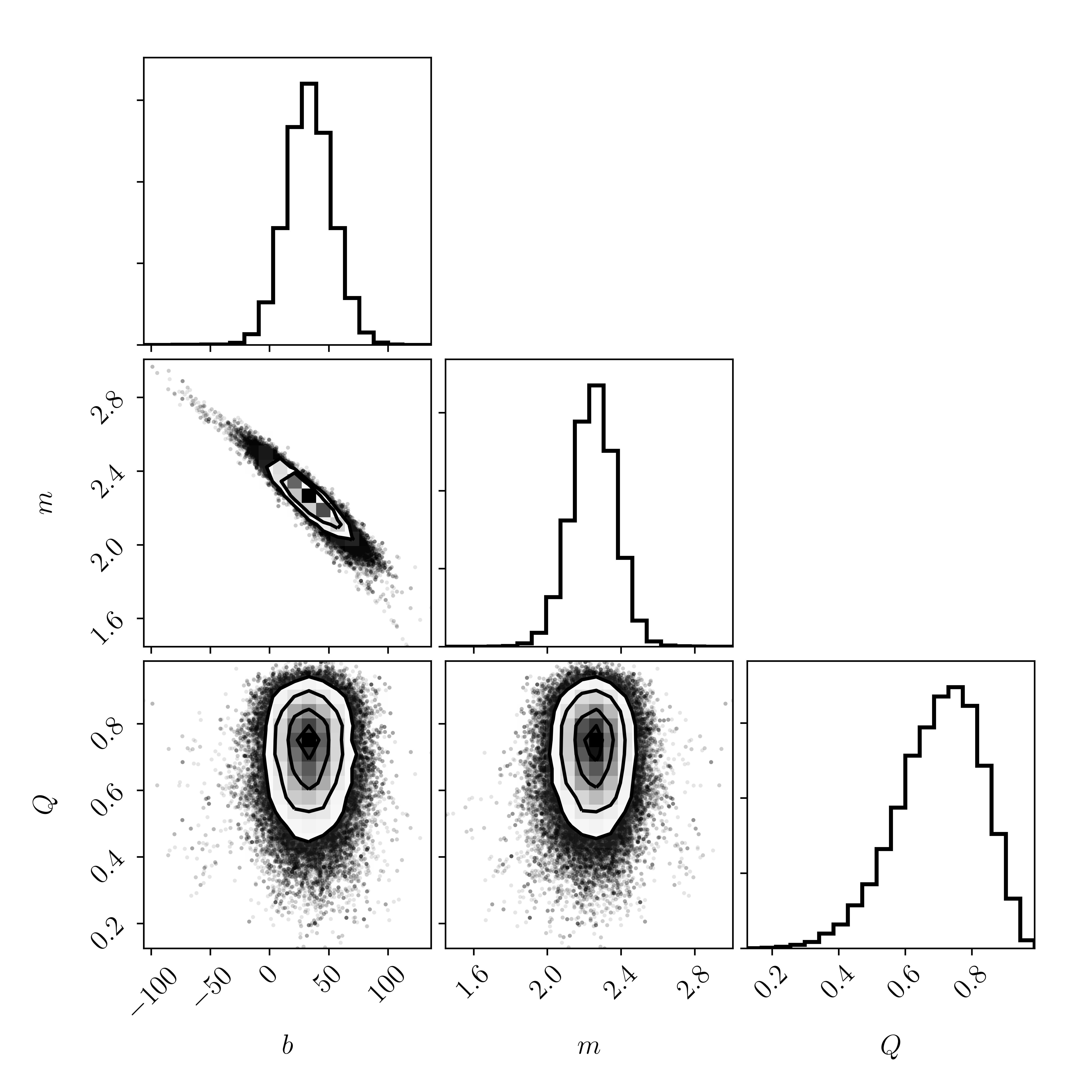
Where here we are only showing a `corner` plot for three of our parameters: \(m\), \(b\), and \(Q\). The parameters of the outlier distribution are so-called nuisance parameters, and we really only care about the marginalised likelihood of the line parameters \(m\) and \(b\), and to a lesser extent, the fraction of non-outliers \(Q\).

Note the scale of these axes. Using linear algebra in the first class the best-fitting model parameters were \(m = 1.07 \pm 0.08\) and \(b = 213.3 \pm 14.4\). The axes of the corner plot above do not even contain those values! Meaning that these posteriors are very different from the solution that we found through linear algebra.
Component membership probabilities
These inferences look sensible, even though they differ dramatically from what we found in an earlier class. The fraction of 'good points' seems to be at around \(Q \approx 0.75\), which seems plausible. So it seems that things look sensible. But what if we want to make some statements about whether an individual point is likely to be an outlier? Let's comment on that before we plot the posterior predictions.
What we actually want is the posterior probability that a data point belongs to the straight line model. That is, we want the probability of \(q_k=0\), given the data: \[ p(q_i|\vec{y},\vec{\sigma_{y}},\vec{x}) = \int p(q_i,\vectheta|\vecdata,\vec{\sigma_{y}},\vec{x})d\vectheta \] \[ p(q_i|\vec{y},\vec{\sigma_{y}},\vec{x}) = \int p(q_i|\vectheta,\vec{y},\vec{\sigma_{y}},\vec{x})p(\vectheta|\vec{y},\vec{\sigma_y},\vec{x})d\vectheta \] This looks a little nasty, but it's not really. In fact, we already have everything we need to calculate this. Before we get ahead of ourself, consider the conditional probability \[ p(q_i|\vectheta,\vecdata,\vec{\sigma_y},\vec{x}) = \frac{p(q_i)p(\vecdata|\vectheta,\vec{\sigma_y},\vec{x},q_i)}{\sum_k p(q_i=k)p(\vecdata|\vectheta,\vec{\sigma_y},\vec{x},q_i=k)} \] which only includes terms that we have already calculated. The numerator describes the posterior for the straight line model, and the denominator is the sum of the posterior probability of both components. But that is given some \(\vectheta\) values, and so we still need to integrate over \(d\vectheta\) \[ p(q_i|\vecdata,\vec{\sigma_y},\vec{x}) = \int p(q_i|\vecdata,\vec{\sigma_y},\vec{x},\vectheta)p(\vectheta|\vecdata,\vec{\sigma_y},\vec{x})d\vectheta \quad . \] However, we have already approximated this integral because we have \(M\) samples from the probability distribution \(p(\vectheta|\vecdata,\vec{\sigma_y},\vec{x})\), so we can just average the probabilities from those samples \[ p(q_i|\vecdata,\vec{\sigma_y},\vec{x}) = \int p(q_i|\vecdata,\vec{\sigma_y},\vec{x},\vectheta)p(\vectheta|\vecdata,\vec{\sigma_y},\vec{x})d\vectheta \approx \frac{1}{M}\sum_{m=1}^{M} p(q_i|\vecdata,\vec{\sigma_y},\vec{x},\vectheta^{(m)}) \] such that \[ p(q_i|\vecdata,\vec{\sigma_y},\vec{x}) \approx \frac{1}{M}\sum_{m=1}^{M} \frac{p(q_i)p(\vecdata|\vectheta^{(m)},\vec{\sigma_y},\vec{x},q_i)}{\sum_{k}p(q_i=k)p(\vecdata|\vectheta^{(m)},\vec{\sigma_y},\vec{x},q_i=k)} \quad . \]
Let's code this up:
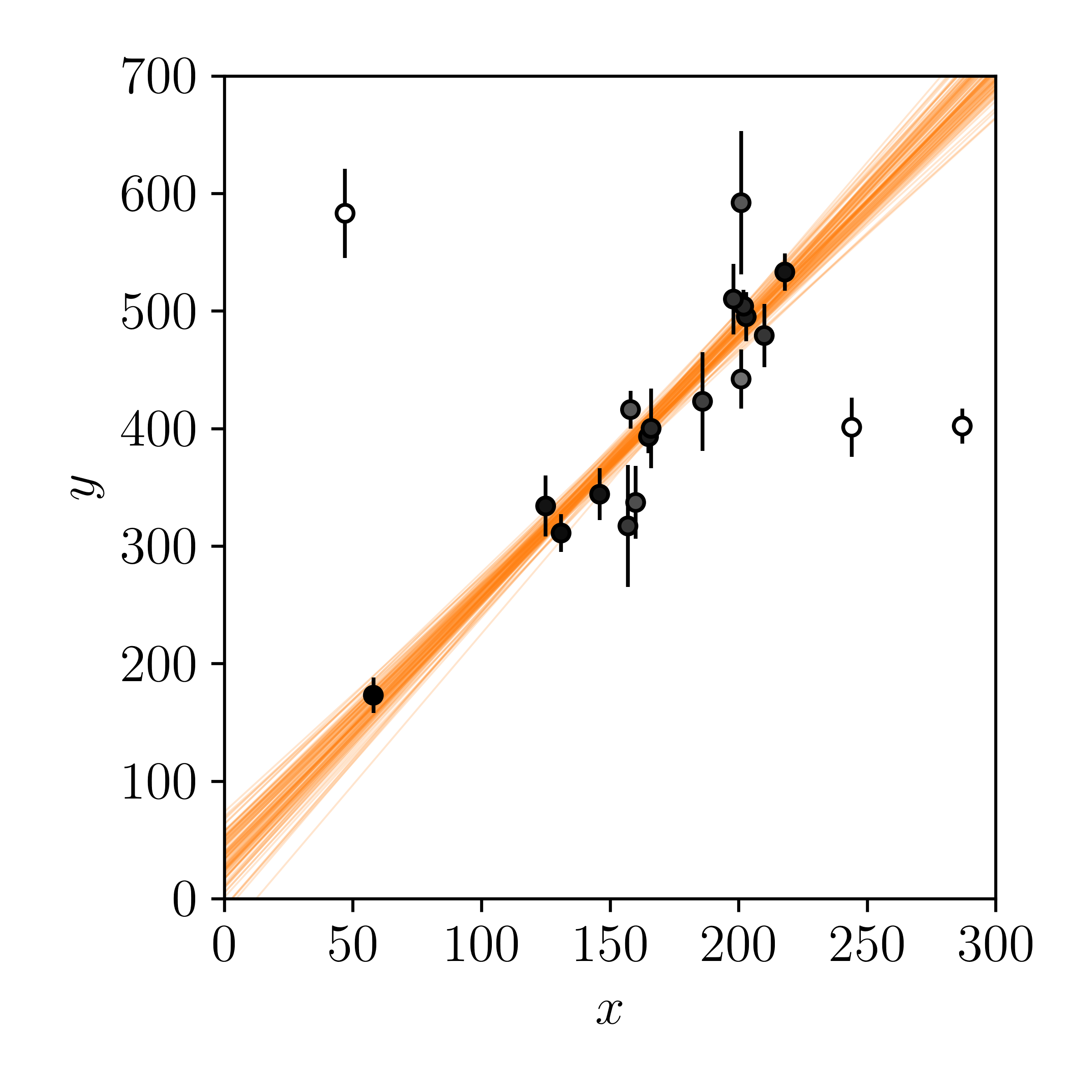
Now we have the \(\vec{q}\) values for each data point, except these are not integers: they are floats that vary from 0 (outlier) to 1 (not an outlier). Let's use these values to shade individual points by their probability of being drawn from the straight-line model, as well as our posterior predictions of the model.

Finally. That looks much more pleasing to the eye.
The process that we went through this week is a typical one for fitting a model to data. Although we have used the most simplistic model (a straight line) as a baseline example, we have explored how complexity can be added. We've covered Bayesian statistics, priors, marginalisation, optimisation, sampling, and posterior predictions.
In the next few classes we will explore optimisation and sampling in detail. These are important topics that are easily abused.