In this class we are going to explore some more complex deep learning architectures that have become popular in recent years. The kinds of networks we will introduce share a common property in that they can be used to reconstruct the inputs given to the network. That might seem foolish at first: why would we want a neural network just to output exactly what it has been given at its inputs? But as you will see, the specific architecture of these networks requires the network to learn the salient features of the input data, and to be able to reconstruct the 'correct' image even if the input data was extremely noisy or corrupted.
The specific networks that we will discuss today are:
- Autoencoders (AEs)
- Variational Autoencoders (VAEs)
- Generative Adversarial Networks (GANs)
And as you will see, these kinds of networks can be very useful in physics and astronomy — or any other field where you care about a probablistic representation of the outputs, or you care about de-noising the inputs. This is a little bit at odds with most parts of machine learning. Normally in machine learning it is common to take the view I care more about what it predicts than how it predicts it, whereas in physics we care more about how predictions are made than the predictions themselves. However, there are some parts of machine learning — commonly referred to as interpretable machine learning methods — where we care just as much about how the prediction was made as to what the prediction is. Machine learning methods that fall into this regime sit in the Venn diagram between "physics" and "machine learning" and can be extremely effective for difficult physics problems.
Autoencoders
An autoencoder is an unsupervised dimensionality reduction technique. Because it is unsupervised, you do not require labelled data for the training set. The general approach of an autoencoder is for it to reproduce the training set inputs. That seems crazy! Why would we feed in a whole bunch of training set data and have it try to reproduce the training set? Wouldn't that just mean that \[ \textrm{output} = \textrm{input} \times 1 \] is an autoencoder? The answer is obviously no, for an important reason. An autoencoder includes a (usually deep) neural network that is structured something like this:
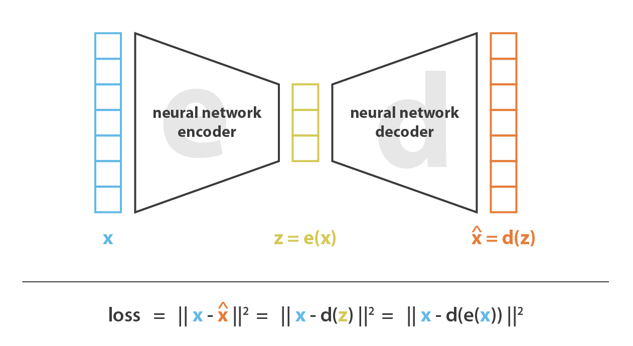
The output block must be the same as the input block, and the network gets increasingly narrow towards the centre of the network. The bottleneck of the neural network — at the central layer — will usually have a very low dimensionality (e.g., 2-5 dimensions). This is a lossy structure, which means that in order for the autoencoder to reproduce the training set it must learn the salient features of the data set and be able to reproduce the entire training set by just moving around in 2-5 dimensions. Since each neuron in the network is able to learn a non-linear mapping, that means this is a non-linear dimensionality reduction technique.
After the autoencoder is trained, you again have two neural networks that can be separated: the encoder (up until the bottleneck) and the decoder (from the bottleneck to the output layer). These could be used in different ways. For example, the encoder could be used to form a highly compressed representation of the data, or to explore how the data are actually compressed (e.g., interpret important non-linear relationships in the data set). Similarly, you could use the decoder as an inference problem: given some new image you are to find the 2-5 latent parameters that best describe that image. Even though these latent parameters are not strictly interpretable, you can take a point in latent space and draw a line in the latent space and see what kind of outputs you get. If you are using an autoencoder on galaxy spectra then you could say "moving in this direction in latent space increases the gas fraction of the predicted spectra". You can do this repeatedly for all the physically interpretable parameters that you want, and then when you use your decoder on new data you can map your latent parameters to physically realistic ones. And you've done all of this without any labelled set!
What's wrong with Autoencoders?
Normally in our data set we will have natural categories of different objects. For the classic MNIST data set this would be images of hand-written digits. But if we were dealing with images of galaxies then their morphological type or orientation would be natural groupings. There may be a continuous representation between these different groups — if we have observed enough objects to map between the different groups — or there may not be. In either case, an autoencoder can end up learning a two-dimensional latent space that looks something like this:
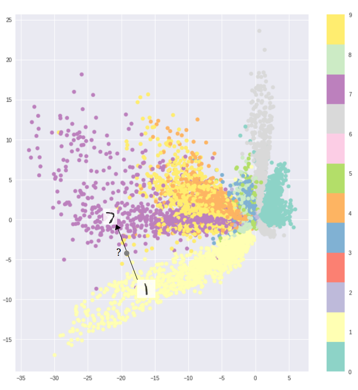
Here we have taken each object in the training set and passed it through the encoder, and plotted the two dimensional representation of \(z\). Even though the training set for an autoencoder does not need labelling, here we have labelled each encoded point by what we know to be the classification. You can see that the autoencoder has learned a representation between groupings, and that representation seems reasonable: as we move up in the y-axis (\(z_2\)) direction we move from 1 to 7, then 7 to 9, then to 4. All of these transitions are reasonably smooth in that we could find a point between this latent space that would make it hard for a human to decide whether the number is a 1 or a 7!
So what is the problem, exactly? Well normally the groupings like this are neither as clear, nor as interpretable. What happens when \(z_1 = -5\) and \(z_2 = 15\)? Here the deoder would generate an unrealistic output because it has no idea how to deal with that part of the latent space! And we can't simply invent those kinds of inputs for the training space, so instead we want to introduce some additional constraint on the latent space so that movements between groups will remain continuous.
Variational Autoencoders
The fundamentally different thing about variational autoencoders
- Change the objective function to include a term that includes the Kullback-Leibler divergence of the latent space \(z\) to a standard normal distribution.
- Instead of having the encoder output a vector \(n\) that represents the latent space, have it output two vectors of size \(n\): a \(n\)-length vector of means \(\vec{\mu}\) and a \(n\)-length vector of standard deviations \(\vec{\sigma}\).
Let's formulate this. We have a training set \(\vec{x}\) consisting of \(n\)objects, which we assume are generated from some latent representation \(\vec{z}\). We want to draw samples from the prior \(p(\vec{z})\) and feed them through the decoder to produce samples from the conditional \(p(\vec{x}|\vec{z})\), given some parameters \(\vec{\theta}\) of the network. We have already said that we want \(p(\vec{z})\) to be a standard normal (for simplicity and continuous interpolation). But how do we train the model? Since our model is probabilistic, if we really wanted to compare the model predictions (given some \(\vec{\theta}\)) to the data we should evaluate \[ p_\vec{\theta}(\vec{x}) = \int p_\vec{\theta}(\vec{z})p_\vec{\theta}(\vec{x}|\vec{z}) d\vec{z} \] This should look familiar to you, and/or scare you. Why? Because it is intractable to integrate over all dimensions of \(\vec{z}\) — particularly to do so at every training step! The posterior density \[ p_\vec{\theta}(\vec{z}|\vec{x}) = \frac{p_\vec{\theta}(\vec{x}|\vec{z})p_\vec{\theta}(\vec{z})}{p_\vec{\theta}(\vec{x})} \] because we don't ever want to calculate \(p_\vec{\theta}(\vec{x})\). Instead we use the fact that our encoder network (which we will call \(q\)) will approximate \(p_\vec{\theta}(\vec{z}|\vec{x})\). For the encoder network \(q\) with parameters \(\vec{\phi}\):
- Inputs: \(\vec{x}\)
- Network: \(q_\vec{\phi}(\vec{z}|\vec{x})\)
- Outputs: means \(\vec{\mu_{z|x}}\) and standard deviations \( \vec{\sigma_{z|x}}\)
And for the decoder network \(p\) with parameters \(\vec{\theta}\)
- Inputs: \(\vec{z}\) — we sample \(\vec{z}\) from \(\vec{z|x} \sim \mathcal{N}\left(\vec{\mu_{z|x}}, \vec{\sigma_{z|x}}\right)\)
- Network: \(p_\vec{\theta}\left(\vec{x}|\vec{z}\right)\)
- Outputs: means \(\vec{\mu_{x|z}}\) and standard deviations \(\vec{\sigma_{x|z}}\) — we sample the prediction for \(\vec{x}\) as \(\vec{x|z} \sim \mathcal{N}\left(\vec{\mu_{x|z}}, \vec{\sigma_{x|z}}\right)\)
such that the log likelihood
That means when we input latent space values to the decoder, we actually have to sample from the means \(\vec{\mu}\) and standard deviations \(\vec{\sigma}\).
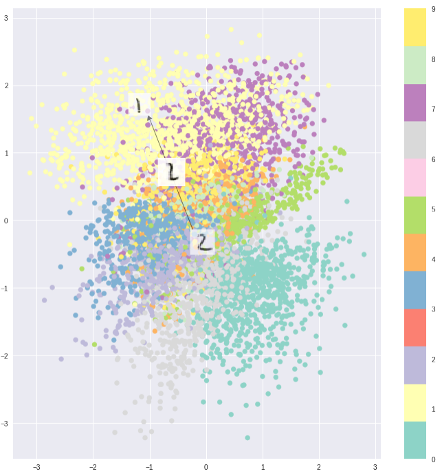
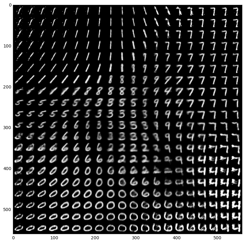
And if you draw samples in the latent space and look at the corresponding (mean) predictions from the decoder, you can see that the autoencoder has picked up on the salient features of each digit, and that the interpolation is smooth and continuous across the latent (and data) space.
Variational autoencoders are therefore particularly good if you have lots of classes of objects in your data set and you want your decoder to make sensible interpolations between the latent space. Variational autoencoders are also very good if you have a training set with varying degrees of noise (e.g., stellar or galaxy spectra) because when you evaluate the loss function you can include the uncertainty in individual data points, and your latent space has some uncertainty with it which preserves the uncertainty in the original training set. And you can propagate any uncertainty in your latent space all the way through the decoder into the output space! That makes variational autoencoders an appealing tool for physics or astronomy problems where we care about preserving and propagating uncertainty.
The primary downside to a variational autoencoder is that your decoder predictions will be noisier than what you would find with something like a GAN. However, a variational autoencoder will have a more interpretable latent space, and be less susceptible to making crazy predictions that are quite unlike the training set.
Generative Adversarial Networks
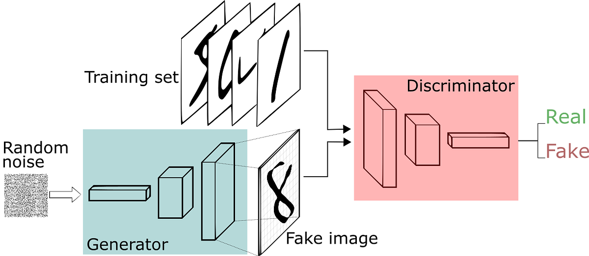
Generative Adversarial Networks (GANs) take a novel approach to training neural networks. Imagine that you would want to sample from a complex high-dimensional distribution, where each dimension in that distribution is a pixel in an image in your training set. If you were able to draw samples from that highly complex distribution, then you would be able to generate images that are like your training set.In this case the images you generate could be ultra-realistic images of people,
The solution that GANs take is to sample from a simple distribution (e.g., a unit normal) of the same size, and then to learn a transformation from that simple distribution to the training set distribution. So our inputs will be random noise, which is then fed through a deep neural network, and the outputs of the neural network should be things that look like our training set.
The key part of how GANs work is that they treat this training process as a two-player game, where you have two neural networks that need training (almost) simultaneously:
- The role of the generator network is to generate images that look real enough to fool the discriminator network.
- The role of the discriminator network is to distinguish between real and fake images.
Initially the weights for both networks are just set randomly. That also might seem crazy because how can either network learn anything if at first the input to the generator network is just noise (so the output will likely be noise too) and the input to the discriminator network is noise (the output from the generator) and some images from the training set. How is either network meant to learn?
We train these networks together in a minimax game. Let us set some defintions:
- \(x\) is the training set of real images
- \(z\) is the input to the generator network
- \(\theta_g\) are the parameters of the generator network
- \(G\) is the generator network, and \(G_{\theta_g}(z)\) is the output of the generator network given the input \(z\) and the network parameters \(\theta_g\)
- \(\theta_d\) are the parameters of the discriminator network
- The discriminator network is \(D\) and \(D_{\theta_d}(x)\) is the output of the discriminator network given the input \(x\) and the network parameters \(\theta_d\). The output of the discriminator network is a probability between 0 and 1 of the input being real.
With these definitions the objective function for both networks is given by \[ \min_{\theta_g}\max_{\theta_d}\left[\mathop{\mathbb{E}}{}_{x\sim{}p_\textrm{data}} \log{D_{\theta_d}\left(x\right)} + \mathop{\mathbb{E}}{}_{z\sim{}p(z)}\log{\left(1-D_{\theta_d}\left(G_{\theta_g}\left(z\right)\right)\right)}\right] \] where it can be seen that the discriminator network \(D_{\theta_d}\) wants to maximize the objective such that \(D(x)\) is close to 1 (real) and \(D(G(z))\) is close to 0 (fake). It can also be seen that the generator \(G_{\theta_g}\) wants to minimize the objective such that \(D(G(z))\) is close to 1 (i.e., the discriminator is fooled into thinking that the image the generator produced is real).
If we take this objective function literally then in practice we should train both networks simultaneously we alternate between performing
- Gradient ascent
Which is the same as performing gradient descent on the negative of the objective function. on the discriminator \[ \max_{\theta_d} \left[\mathop{\mathbb{E}}{}_{x\sim{}p_\textrm{data}}\log{D_{\theta_d}\left(x\right)} + \mathop{\mathbb{E}}{}_{z\sim{}p(z)}\log\left(1-D_{\theta_d}\left(G_{\theta_g}\left(z\right)\right)\right) \right] \] - Gradient descent on the generator \[ \min_{\theta_g}\mathop{\mathbb{E}}{}_{z\sim{}p(z)}\log\left(1-D_{\theta_{d}}(G_{\theta_g}\left(z\right)\right) \]
However when the sample \(D(G(z))\) is likely fake (e.g., \(D(G(z)) \approx 0\)) we want it to improve the generator, but the gradient of the generator function is relatively flat when \(D(G(z)) \approx 0\):
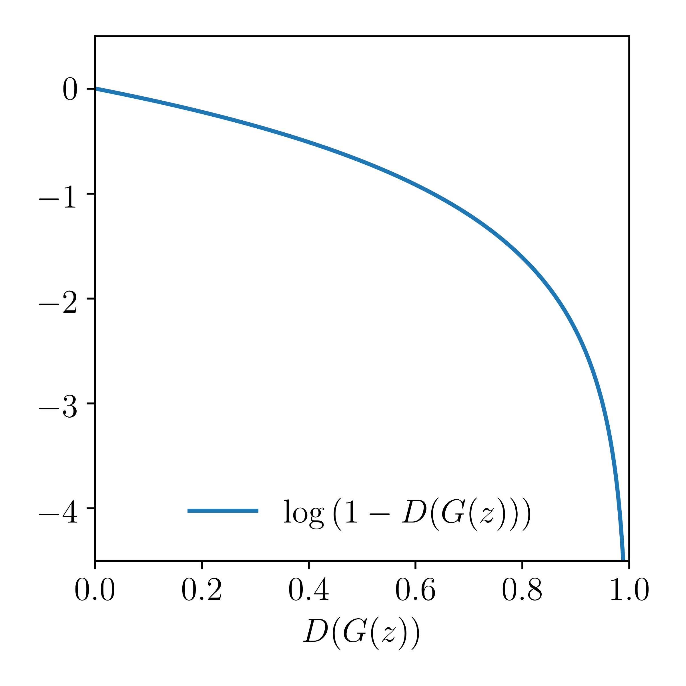
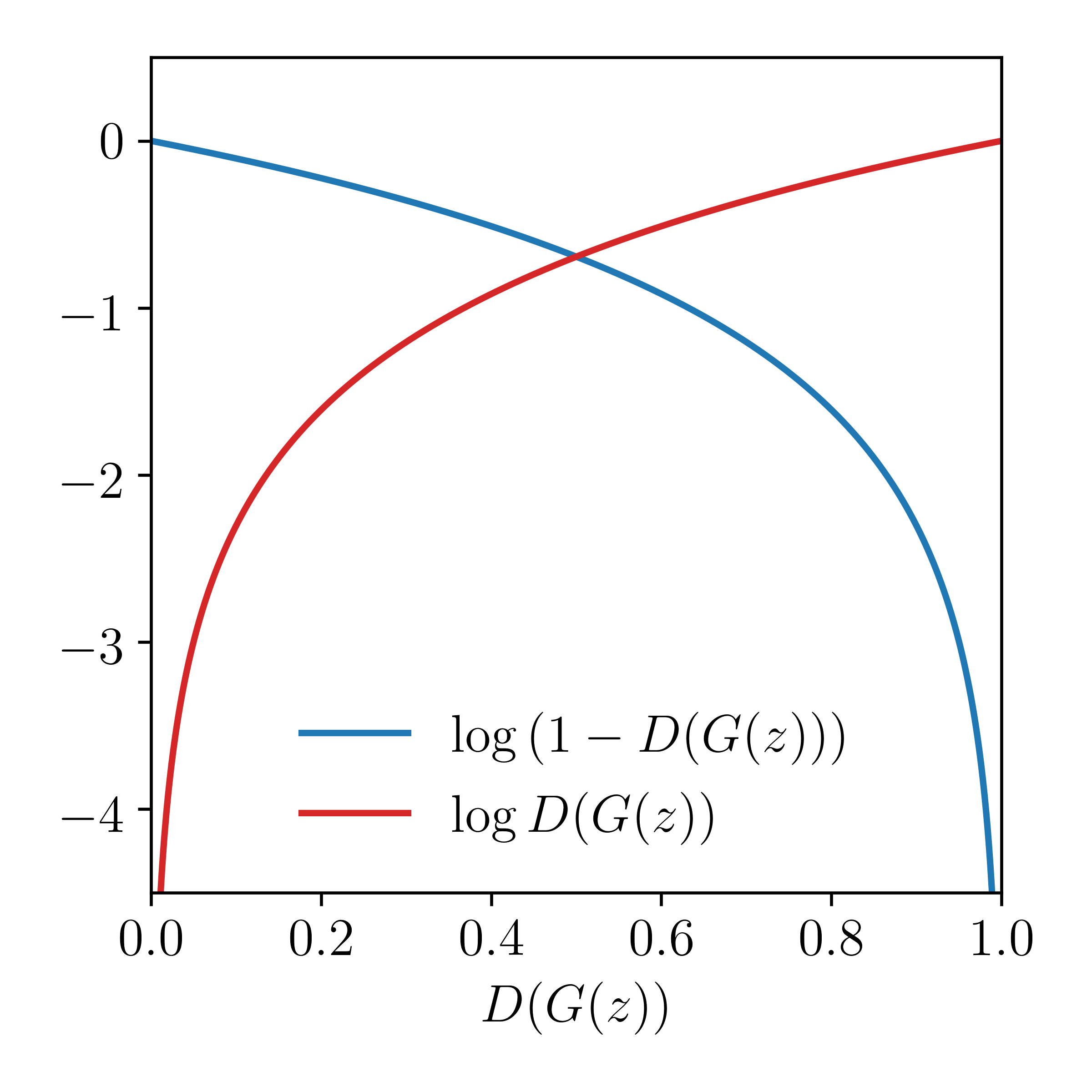
So instead we perform gradient ascent on the generator with an objective function that has a higher gradient for bad samples.
So in practice we alternate between performing
- Gradient ascent on the discriminator objective \[ \max_{\theta_d} \left[\mathop{\mathbb{E}}{}_{x\sim{}p_\textrm{data}}\log{D_{\theta_d}\left(x\right)} + \mathop{\mathbb{E}}{}_{z\sim{}p(z)}\log\left(1-D_{\theta_d}\left(G_{\theta_g}\left(z\right)\right)\right) \right] \]
- Gradient ascent on the generator objective function \[ \max_{\theta_g}\mathop{\mathbb{E}}{}_{z\sim{}p(z)}\log\left(D_{\theta_{d}}(G_{\theta_g}\left(z\right)\right) \]
If you are having trouble imagining a GAN, consider that you have some set of money notes and the setup is as:
- The generator network is a counterfeiter that wants to learn how to produce realistic looking notes. They can't really just make notes that they think are good enough, because in the end the notes they produce are only 'good enough' if someone else is willing to accept them, or better yet, if the police believes they are real!
- The discriminator network is the police. They have some set of \(2\times{}m\) notes: \(m\) produced by the generator and \(m\) real notes. But the notes got muddled up, so they don't know which notes came from the generator and which notes were real. The discriminator's job is to decide which notes are real, and which notes are fake.
At the start of training neither network will perform very well. After a few iterations it will be clear to the discriminator as to what looks like a real note, and what looks like fake images produced by the generator.
At this point you have two useful neural networks. The discriminator could then be separated from the GAN architecture and used on its own to discriminate between real notes or fake notes. And since the discriminator has gone through many trials with a generator randomly trying to fool it, you will have a pretty good discriminator! Similarly, you can now separate the generator network from the GAN and use it on it's own. Remember that the generator is taking random draws from a unit normal as inputs and producing realistic pictures of money each time! That should be incredible to you. If it's not: recall that the generator is not chosing images to produce from the training set — the generator has never explicitly seen what is in the training set, or what a note looks like! Your generator has only ever been given random noise as inputs, and it has only been told (inadvertedly, through gradients) whether the output it provided was a real-looking note or not. If it's still not remarkable to you,.. the training set images could contain anything: videos, audio, pictures of people, animals, landscapes, paintings, et cetera. For any of these kinds of data, a GAN could
GANs with convolutional architectures
Imagine if the generator in our GAN only included dense, fully connected networks. We may be generating pictures of notes, but we are going to have a real problem in scaling this up to large high resolution images. That's because in our dense fully connected network if one pixel has a reddish colour (consistent with a 20 dollar note) then there's no joint constraint that the neighbouring pixels should also have a similar colour. But in practice we would expect that of any photo taken of a note, particularly if it is low resolution! For this reason it is common to have convolutional architectures in generator networks, such as this:
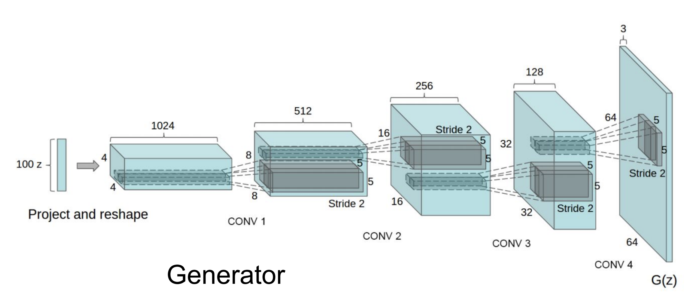
With this kind of architecture we will draw from a 100 dimensional unit normal distribution \(z\), which goes through a series of convolutional layers to predict a \(64\times{}64\) pixel image (4,096 size instead of 100). The end result is that random draws in \(z\) produce more photo-realistic images, and interpolating between places in \(z\) produce smooth — albeit unusual to look at — changes in the output images (e.g., from having desks in a room to having no desk, adding glasses on peoples' faces, et cetera).
Interpretable vector math
By tracing directions in the latent space \(z\) we can also come up with causal explanations for what that vector means. For example, imagine if you could find a line through the latent space \(z\) where, no matter how you sampled along that line, the generator only produced images of men wearing glasses, which we will call set \(A\). Now imagine that you found another line that only produced images of men not wearing glasses, \(B\). Then another line that produced images of women not wearing glasses \(C\)
- \(A\): men wearing glasses
- \(B\): men not wearing glasses
- \(C\): women not wearing glasses
Many GAN architectures available
There were many problems with the vanilla GANs. These were mostly due to optimisation problems, but they led to serious concerns about how applicable GANs could be for Real World™ problems. Now there are many variations of GANs around, which have uncanny abilities to produce new images of people and places that do not exist.
Summary of GANs
They do not have an explicit density function. Instead they use a game-theory approach to train two neural networks simultaneously. It is a very novel idea that produces beautiful samples. The downsides are that they can be extremely tricky or unstable
Summary
You can combine neural networks in counter-intuitive ways that can be used to de-noise data sets (e.g., GANS), or make them separable so that they can be used for different tasks after training. And through certain structures of neural networks, we can make them probabilistic and have their latent space be interpretable (e.g., VAEs). This makes them appealing to problems in physics and astronomy, where we may have lots of unlabelled and noisy data and we want to perform inference!