Now that you have some background on how a neural network can be built up from scratch, it is time to introduce you to additional components that are commonly used in neural networks. So far we have only considered neural networks to have fully connected (FC) layers, where all neurons have connections to all other neurons in the neighbouring layer. We have also only considered using neural networks for regression, where we are interested in predicting the quantity of something (e.g., house prices) given some input data. But anything that can be used for regression can also be used for classification!

In this lecture you will be introduced to a few different components of neural networks:

Together these components can be used to build Convolutional Neural Networks (CNNs), which are popular in for general image processing problems, and for image problems specific to physics and astronomy. We will go through some example uses in physics at the end of this lecture.We will also cover some of the practical steps associated with training a CNNThings like data augmentation which are applicable to all neural networks, but particularly critical for CNNs. like data augmentation and feature optimisation, and caveats like adversarial attacks.

Neural network components

Softmax functions for classification

If we are interested in classifying things with a neural network, instead of predicting continuous properties, then there is not much we have to change to the network. The only thing we usually have to change is the output layer. There we will want to introduce something like the Softmax function so that our output predictions are converted to (something akin to) probabilistic classifications, \[ \sigma\left(\vec{z}\right)_i = \frac{e^{z_i}}{\sum_{j=1}^{K}e^{z_j}} \] where here \(\sigma\left(\vec{z}\right)_i\) is the softmax function for the \(i\)-th input and \(\vec{z}\) is the set of \(K\) inputs to that function. You can see that this function will take in all the input predictions and normalise it to a probability distribution where the sum of all probabilities will be equal to one. We should not truly think of this as a set of probabilities per se because most neural networks have no concept of probability, uncertainty, variance, or anything even remotely similar! Instead you can think of the outputs of the softmax function of being some relative degree of belief from the network as to the classification of a single object. In other words, if one softmax output is higher than another then the network believes that output to be more probable, but the difference in those two outputs is not proportional to the true probability of belief.But if it's all you've got, you take it!

Convolution kernels

Imagine you have been given a data set of images that are 32 pixels by 32 pixels in size. Each image has three channels — red, green and blue — that record the intensity in each channel. Your task is to design a neural network to make a single binary classification.

How many inputs would you have going in to each neuron if you were to use a fully connected hidden layer? \[ N_\textrm{inputs} = 32\,\textrm{pixels} \times 32\,\textrm{pixels} \times 3\,\textrm{channels} = 3072\,\textrm{weights} \] That's 3072 weights (and a bias term) for every neuron in your first layer. Even if you had just 10 neurons in your first layer, you already have \(\sim{}30,000\) parameters in your network. That's fine — too many parameters is not necessarily a road bloack — the problem is that too many of your parameters are redundant.

For example, there is a lot of spatial information in the image that is entirely ignored by having a fully connected network. Nearby pixels will share information about the object in the image, but when you provide the input data to a fully connected network it has no concept of which pixels are spatially close to each other, or what the value of each input actually represents (e.g., that input 23 is the red channel of one pixel and that input 24 is the blue channel of the same pixel). In this kind of situation a fully connected network is like trying to hit a mosquito with a cannonball. It's overkill, and it probably won't work.

Instead we will structure the input data not as a column vector of individual values, but a volume (or matrix) of data where the sizes of the input matrix have physical meaning. In the case of an image our input data volume might be \((N_\textrm{images}, 32, 32, 3)\). The rest of the components of the network will be similarly multi-dimensional, with the dimensionality set to represent physical characteristics about the dataset.

With the input data structure set correctly, now let's introduce convolutional layers. A convolutional layer describes a set of learnable filters, where each filter is usually small on a spatial scale (e.g., width and height) but has the same depth as the input volume. Filters for use on images will usually have a shape like \(5\times5\times3\): 5 pixels wide, 5 pixels high, and one for each channel. Consider a \(2\times2\) convolution for a single channel, where the data are in blue and the convolution result is in green. The simplest case is where we have no padding and no strides (top left).

Animations by Vincent Dumoulin and Francesco Visin (see here and here).

As we slide the filter over the image we produce a map that gives the response of that filter at every spatial position. Those maps can be spatially smaller than the input map (as above), or the input data can be zero-padded to ensure the output map has the same size map, or even a larger map. Zero-padding is not just a numerical trick: it is used to ensure that information at the edge of images has the same potential importance as pixels at the centre of the image.

We can also chose to stride the filter over the image to set the structure of the filter output. In the above animations we are using no stride, such that we are just stepping one pixel at a time. When we use a stride of 1 we are 'jumping over' one pixel at a time. We are not necessarily losing information by striding, though, if our filter size is large enough.

You could imagine taking a fully connected layer and then cutting many of the connections until you only have neurons being fed information from neighbouring pixels together. Indeed, convolutional layers are nothing more than using domain expertise to allow certain neurons to be connected, while disallowing others. Here is another animated view of how a kernel filter works, with some numbers:

But what values does the kernel take? The values of the kernel are learnable weights in the network, but you can imagine a few kinds of kernels that emphasize certain features in an image (e.g., see this interactive post for examples, or basic edge detection). If you have particular domain knowledge then you may want to forcibly set the kernel weights for one neuron (e.g., to perform a Laplacian or Sobel operation), but usually we would want the network to learn the best filter representations from the images that will predict the best outcomes.

When setting up a convolutional layer you need to be aware of the input volume size \(W\) the stride length \(S\), the filter size \(F\), and the amount of zero-padding \(P\) used. These quantites will set the shape of your convolutional layer(s). For example, for a \(32\times32\) image (single channel) and a \(5\times5\) filter with stride length of 1 and zero padding of 1 we would expect a \(29\times29\) output from the filter. The number is given by \[ \frac{W - F + 2P}{S} + 1 \] along any axis. Your filter size, stride length, etc are all hyperparameters for a given convolutional layer, but they have mutual constraints. For example if you have an input image of size \(10\times10\) with no zero padding and a filter size of \(F=3\) then it is impossible to use a stride length of 2 because it does not given you an integer number of outputs.

Let's show an example in numpy so that you can see how the filter outputs relate to the basic idea of a neuron. Let us state that we have some square input dataX that has a size \(5\times5\) (\(W = 5\)), and depth (or number of channels) of 3. We will use a zero padding of 1 (\(P = 1\)), set the filter size as \(F = 3\), and set the stride to be \(S = 2\). The output map should have spatial size \[ O = \frac{W - F + 2P}{S} + 1 = \frac{5 - 3 + 2(1)}{2} + 1 = 3 \] and in our code we will call the output volume V. We will denote the weights of the kernel to be w0 and w1 and the bias terms to be b0 and b1. import numpy as np np.random.seed(8) # Data. W, D_in = (5, 3) # input image sizes x_original = np.random.randn(W, W, D_in) # Hyperparamters. F = 3 # filter size S = 2 # stride length P = 1 # zero padding # Outputs D_out = 2 # We assume! O = int((W - F + 2 * P)/S + 1) o = np.empty((O, O, D_out)) # Filter weights and biases. w0 = np.random.randn(F, F, D) w1 = np.random.randn(F, F, D) b0, b1 = np.random.randn(D_out) # Zero-pad the data. x = np.zeros((P + W + P, P + W + P, D_in)) x[P:W+P, P:W+P, :] = x_original[:] # Do first row of first channel. o[0, 0, 0] = np.sum(x[0:3, 0:3, :] * w0) + b0 o[1, 0, 0] = np.sum(x[2:5, 0:3, :] * w0) + b0 o[2, 0, 0] = np.sum(x[4:7, 0:3, :] * w0) + b0 # Do first column of first channel. o[0, 0, 0] = np.sum(x[0:3, 0:3, :] * w0) + b0 o[0, 1, 0] = np.sum(x[0:3, 2:5, :] * w0) + b0 o[0, 2, 0] = np.sum(x[0:3, 4:7, :] * w0) + b0 # ... keep going ... # Do first row of second channel. o[0, 0, 1] = np.sum(x[0:3, 0:3, :] * w1) + b1 o[1, 0, 1] = np.sum(x[2:5, 0:3, :] * w1) + b1 o[2, 0, 1] = np.sum(x[4:7, 0:3, :] * w1) + b1 # Et cetera. You obviously want to do this by # matrix multiplication, but here you can see # how the inputs relate to typical weights and # biases in a FC layer.

The entries in the output volume are then fed to an activation function (e.g., ReLU). You can visualise this process in the following animation:

Often it is common to keep filter sizes small (e.g., between \(3\times3\) or \(7\times7\)) and to have many convolutional layers that keep convolving the image rather than having one convolutional layer with a very large filter.Why do you think this is? That necessarily implies that as soon as you start getting images that are reasonably large in size (e.g., \(2048\times2048\)), you are going to have a very deep network! The purpose of those convolution layers is to learn non-linear relationships in the data, and to impose spatial structure in those non-linear relationships. Essentially you are trying to train the weights in the filters such that they highlight (or engineer) features in the data. At the output of all those convolutional layers it is typical to find a fully connected (FC) layer (or many!) before the output layer.

Pooling Layers

The last component that you need to know about is that of a pooling layer. Usually you would insert a pooling layer between successive convolutional layers in a network, where the pooling layer just reduces the spatial size of the repesentation to reduce the total number of convolutional layers you need. Unless denoted otherwise, normally when we describe a pooling layer we are describing it as taking the maximum value of some number of spatially neighbouring inputs.

3x3 max pooling over a 5x5 feature map. Pooling layers are used to reduce the spatial size of a feature maps without using a convolutional layer. A pooling layer has no neuron weights or biases, so it is computationally efficient.

Convolutional Neural Networks

The network architecture we have been largely describing is exactly that of a Convolutional Neural Network (CNN): many convolutional layers, with some fully connected layers, to learn non-linear relationships in the data that where spatial structure is a must. CNNs are extremely popular for image classification tasks.

There are some important things to consider because e are forcing the network architecture to learn spatial relationships. Imagine if your training set included images of either peoples' faces, or houses. But imagine that every house image you supplied to the network was upside down. If you trained a convolutional neural network and then gave it an image of a house that was right-side up it would probably tell you that the image was a human face. This is because the network will learn any non-linear mapping that best describes the separation of different classes. It is not learning what a window is, or what a nose is, or anything of that sort. It will pick up on the largest differences between the two data sets, because that is where the gradient tells it to go!

For this reason it is important to perform data augmentation when training neural networks. Data augmentation can be useful for fully connected networks too, but it is critically important for convolutional layers. Data augmentation is a process where you either supply the same training set multiple times (with different operations applied to it each time), or you give the same training set and you apply random operations to each image. Usually it is the former: you provide the same training set multiple times. Each time you are supplying an observation to the training set you perform an operation on the image to prevent the network from picking up on features that you don't want it to. This could include:

The exact set of operations (and how frequently you perform them) depends on the data set and the problem at hand, and whether you care about specific operations or not. For example, when identifying galaxies we are not interested in the particular orientation of the galaxy with respect to Earth. 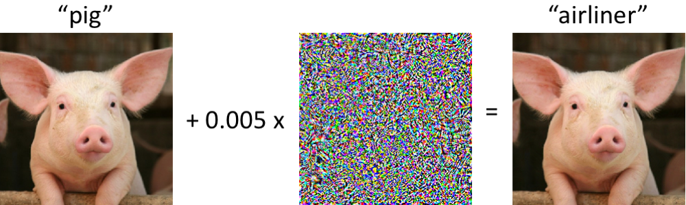So in that case we could flip the image left-to-right or up-to-down, or we could rotate the images (if we were willing to live dangerouslySee previous footnote!). Alternatively, if we were using a CNN to look for gravitational lensing of galaxies then we may want to take a sample of normal, unlensed, galaxies and apply many different random lensing effects to those galaxies. We may want to do this many, many times so that the neural network picks up on features of lensing rather than features of galaxies.

Data augmentation can be useful for protecting CNNs against adversarial attacks, particularly if you are performing data augmentation by adding lots of noise effects. An adversarial attack is one where you can change an input image ever so slightly — either in the form of a single pixel being a different value, or by adding small amounts of noise in a particular pattern that would be indistinguishable for a human — and drastically changing the output prediction of the neural network.

An example of an adversarial attack where a CNN correctly classifies an image of a pig (left), but after adding indistinguishable noise to the image the CNN classifies it as an airliner [source].

The early days of CNNs were used to classify an object (or digit, et cetera) in an image. That meant that your output layer was single-width, and maybe only a few categories (only a few neurons). That works well for simple problems, but for more advanced problems we want a different architecture. For example, we may want to better understand why a network is predicting something, or where in the image is it identifying the object we are interested in. That kind of question is very different to that of "is there a toaster in this image?" because knowing where objects are in an image, and what those objects are, enables automation in things like self-driving cars, et cetera.

U-Nets

Introducing U-Nets. A U-Net is a particular kind of convolutional network where the output layer has an equal shape (or scaled shape) as the input data. The typical architecture looks something like this:

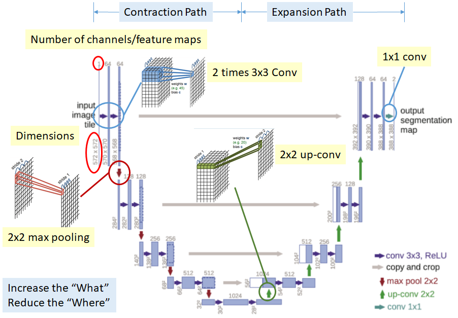
Here the outputs of the network are predictions at every pixel for whether that pixel contains an object of interest, or not. The depths in the output layer may be things like car, or person, or galaxy. That is to say rather than using a CNN to predict is there a person in this image? it is tasked at saying show me the pixels that contain people in this image. The predictions maps are called saliency maps, for which you can use basic image processing techniques to group nearby pixels together and to count the number of people, or to put boxes around each person, et cetera. To ensure the architecture shape works correctly, U-Nets have a series of up-sampling steps (opposite of the convolutional steps) after the set of FC layers. U-Nets have become extremely popular in many fields because you can use them to understand whya neural network is making certain predictions: because you can see where it believes an object is in the image, rather than just saying it thinks there is an object in the image. U-Nets have also been described as fully convolutional networks, but U-Net is more common.

Uses in physics and astronomy

CNNs have become very popular in physics and astronomy, as they have in other fields. This includes classical CNN structure where you want to classify objects, and U-Nets where you want to identify many objects in images. Just from searching for papers in the last year you will see that convolutional neural networks have been used to:

Summary

Convolutional Neural Networks are just a special way of enabling and restricting certain neurons from a fully connected layer, such that it forces the network to learn non-linear mappings in the data that has spatial structure. This kind of structure is particularly good for images, or situations where you expect data to be correlated between observations (e.g., one dimensional time series). Through a series of convolution layers, down- and up-sampling, and pooling, you can construct a network that efficiently makes predictions. And although we didn't cover it explicitly here, you can use pre-trained CNNs that were trained on different data, and re-train them with your dataset of interest! This is almost certainly the norm these days, rather than going through the pain to train your network from scracth.

In the next class we will go through architecture of neural networks that incldue memory, which will conclude our discussion about the components that modern neural networks are currently build from.


No padding, no strides	Arbitrary padding, no strides	Half padding, no strides	Full padding, no strides

No padding, strides	Padding, strides	Padding, strides (odd)

Neural networks III