By now you should know a bit about how neural networks are structured and what goes in to training them. Now we will go through their components in detail, and introduce critical concepts you will need to know in order to efficiently train a network.
Activation functions
In the last class we used a sigmoid as our activation function. We also introduced you briefly to the Rectified Linear Unit (ReLU) activation function. For both of these activation functions we explained some bad attributes about them. Sigmoid functions will have vanishing gradients when they saturate, which can kill off part of your network. Similarly, if a ReLU unit does not have a constant small signal going through it during training then you may end up with a dead neuron with zero gradient!
There are benefits and disadvantages to every activation function. Here are some common ones: activation function plots
Sigmoid
The sigmoid function \[ f(x) = \frac{1}{1 + e^{-x}} \] will squash input numbers to be between zero and one. Sigmoid functions have historically been popular because they have a nice interpretation of 'activating a neuron'. But you can see that this is where the neural analogy has failed us, because using backpropagation with sigmoid functions can result in vanishing gradients very easily.
Disadvantages:
- Saturated neurons 'kill' gradients.
- Sigmoid outputs are not zero-centered, but we zero-center our data! That seems inflexible..
- Weights will always be all positive or all negative.
- \(\exp{}\) is (relatively) expensive
Hyperbolic tangent function
The hyperbolic tangent function \[ f\left(x\right) = \tanh{\left(x\right)} \] is often used as an activation function. It's good because it squashes numbers to between -1 and +1, which means it is zero-centered (good, just like our data). Unfortunately, like the sigmoid function, it still kills gradients when saturated.
Rectified Linear Unit (ReLU)
The ReLU function \[ f\left(x\right) = \max\left(0, x\right) \] is a very simple and effective activation function. If you care about the analogies to neurons, then a ReLU is probably a slightly better approximation to neuron connectivity than a sigmoid function. It also has other advantages:
- Does not saturate for any positive \(x\) value.
- Much more computationally efficient than \(\exp{}\) or \(\tanh{}\).
- In practice it converges much faster than sigmoid or hyperbolic tangent functions.
The only problems with ReLU units is that they do not produce zero-centered outputs, and you can end up with dead ReLUs if they are never activated. In practice many people initialise their weights such that all ReLU units will have a small bias term to begin with to avoid dead neurons.
Leaky ReLU
This is very similar to the ReLU, except with one small change to avoid having dead neurons. The Leaky ReLU is defined as \[ f\left(x\right) = \max{\left(0.01x, x\right)} \quad . \] It has all the other benefits of a ReLU (e.g., faster convergence, cheap, et cetera), except they will not die. Their downside is still that they don't have zero-centered output.
Parametric Rectified Linear Unit (PReLU)
Now we are just naming things. This is just like a Leaky ReLU except we replace the arbitrary 0.01 value with a term \(\alpha\), which you can backpropagate through your network \[ f\left(x\right) = \max\left(\alpha{}x, x\right) \quad . \]
Exponential Linear Units (ELU)
An Exponential Linear Unit is defined as \[ f\left(x\right) = \left\{ \begin{array}{ll} x & \quad & \textrm{if} x > 0 \\ \alpha\left(\exp{\left(x\right)} - 1\right) & \quad & \textrm{if} x \leq 0 \end{array} \right. \] and has all the benefits of a ReLU. It has a negative saturation regime compared to Leaky ReLU, but the computation requires \(\exp{}\) which is expensive.
Summary of activation functions
There are many activation functions available. Here's the summary of what you need to know:
- Try sigmoids.
- Try hyperbolic tangent functions.
- Try out Leaky ReLU / ELU / PReLU.
- In the end: Use ReLU but make sure you initialise the weights such that you have a slight positive bias for all neurons, and make sure you are careful with your learning rate.
Keep it low to be slow, and sure.
Normalising the data
This step is also referred to as preprocessing the data, and you do it in at least two stages:
- You calculate the empirical mean and variance (and perhaps some translation) of the input data, and record those values.
Because you will need them later! - After taking the predictions from your network, you multiply your predictions by the square root of the empirical variance you calculated earlier, and add the empirical mean you calculated earlier.
Basically you are making sure that the data that goes in and through the network is zero-mean and nearly unit variance. You apply the a transformation to data going in to the network to make it zero-mean and unit variance, and then you apply the reverse transformation on your network predictions to bring them back to the right data scale. But why would we want to have the input data as zero-mean and unit-variance? Imagine what were to happen if we didn't! Imagine if we had very large input \(x\) values, say \(\sim{}10^6\). We would need our weights to be very small (\(\sim{}10^{-7}\)) otherwise we would immediately saturate our first layer of neurons. And even if we didn't immediately saturate them, we would need extremely small learning rates because the initial weight might be something like \(w = 10^{-6}\), and if the gradient is non-zero then we only want to be making tiny adjustments to the weight values through backprop otherwise a non-tiny adjustment, when multiplied by the massive input values of \(\sim{}10^6\), will saturate the neurons.
So zero-centering and adjusting the variance is important. Often you may also see people doing Principal Component Analysis on the input data so as to de-correlate it and whiten it before feeding it to the network. This is also fine to do, as long as your network will not be losing information about correlations between the two input variables.
Now consider what happens as our whitened data flows through the network. Indeed, imagine if we had many layers in our network — something like ten or more. No matter how we initialised our weights, and how we pre-processed the data, then by the last layer you will find that the inputs to the last layer will not be zero-mean and unit variance. Just through the flow of data all throughout the network, you might expect to find a very different distribution for the inputs to the last layer of your network. That's good in a way because our network will adjust weights to learn relationships in the data, but it can be very bad if we really want the inputs to all layers to have zero-mean and unit variance. For this reason it is common to find people doing something called batch normalisation.
Batch normalisation is where the inputs to all neurons in a layer will be normalised to have zero-mean and unit variance. That is to say that we perform normalisation every single time before the activation function. With each step we need to record the empirical mean and variance of all the inputs going in to the network, so that we can translate the data appropriately later on. It might seem like a crazy idea to do this, but you should be able to imagine that it will massively improve the gradient flows through the network (e.g., the learning process, since it relies on backpropagation). Because the gradient flows are more stable you can use higher learning rates than you otherwise would, and it reduces the dependence on initialisation. So if you have a deep fully connected network, or you have convolutional layers in your network, batch normalisation is usually a good thing to do.
Initialising the weights
We have hinted at the fact that initialising the weights correctly is important. If we initialise them too high then we will saturate sigmoid neurons. If we initialise them too low then we will kill off ReLU neurons. If we initialise them wrong (in some other way) then it will take longer to train our network. So how do we initialise them?
Imagine the network that we looked at in the previous class. What were to happen if we just set all weights to be at the same constant value?
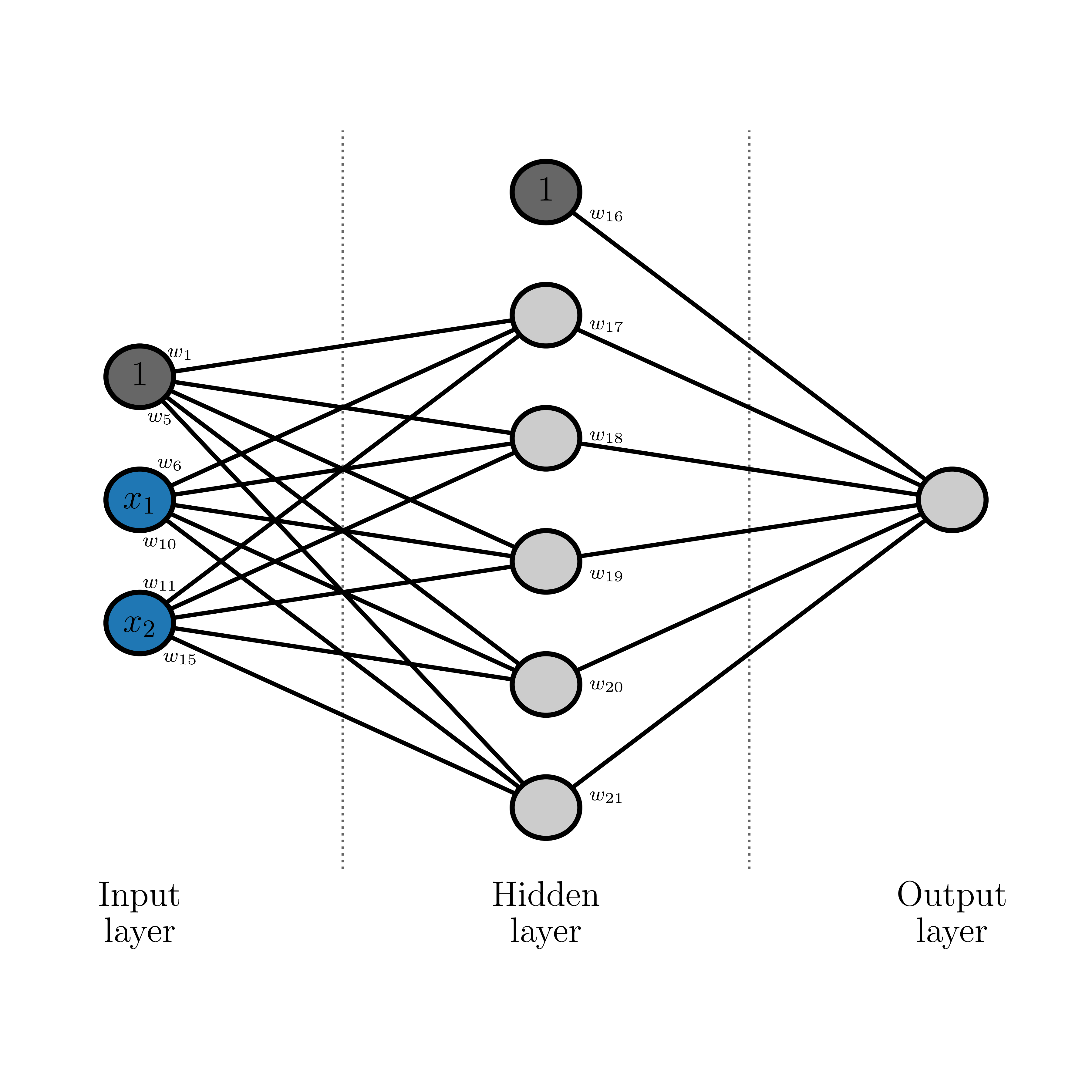
You can imagine that if the constant weight value were high enough, you would activate some neurons in the first layer. And then since those neurons are activated (i.e., have a high value) then when they are multiplied by the constant weight value to go to the next layer then even more neurons will become activated. And so on and so forth. That means for a constant value for all weights, we are more likely to activate (and saturate) neurons that are in deeper layers in the network than we are for those neurons in the first layer. You might not think that is a bad thing, but it is.
If the constant value were lower, what would happen then? Imagine the data flowing through the network in the same way as we just considered. Now, instead, we are far more likely to have neurons at the end of the network be zeroed-out than those in the initial layers. This is even worse, since if most neurons in the last layer are zeroed out then it means those vanishingly small gradients will flow back through the network and affect the weights for all neurons. In short, it will kill off the training because there are no gradients available to update the weights. Or network will never learn!
If you are using zero-centered and unit-variance data inputs then it is normally sufficient for you to draw your weight initialisation as
\[
w \sim \mathcal{N}\left(0, 1\right) \quad .
\]
This will work fine for small networks. But for deep networks we will have problems, as we alluded to above. One way to address this is to scale the width of the normal distribution relative to the number of inputs to that neuron. So if you have a layer of neurons with \(W_{in}\) inputs to the layer, you would initialise the weights in that network as
\[
w \sim \mathcal{N}\left(0, \frac{1}{\sqrt{W_{in}}}\right)
\]
where \(W_{in}^{-1}\) represents the variance in the distribution you are drawing from, and \(W_{in}^{-\frac{1}{2}}\) represents the standard deviation. This kind of initialisation will work very well for sigmoid functions, but will actually fail for ReLU activation functions.
Instead, for ReLU activation functions, you can use something like
Regularisation
We have covered regularisation before in our introduction to machine learning. Regularisation is often used in neural networks to force weights to zero unless they have to be. This, and other techniques like dropout, are useful for ensuring that neural networks do not over-fit the data. Since we know that neural networks are universal interpolators, that means they can literally reproduce any data set, which means they will be prone to overfitting the data set you give them unless you are careful.
Tips for regularisation in neural networks is the same for standard data analysis. You will normally use a \(L_2\) norm (since your problem is non-convex already) and usually you will use a single regularisation strength. That regularisation strength becomes a hyperparameter that you need to solve for, for your network. The standard approches remain good ones: start with a small regularisation value, and trial increasing values on some grid that is uniform in log space. When your regularisation strength has gone too high you will see it immediately in your loss rate: at increasing epochs (even in the first few epochs) you will see your loss function increasing with time instead of decreasing!
A more common way of managing overfitting is through a technique called drouput. That is where each neuron has a probability of being zerod-out in some forward pass. When we randomly drop out individual neurons in each pass it makes the output noisy, and subsequently makes the gradients noisy. That means if you are using dropout you will need to set a hyperparameter for the probability of dropping out a neuron, and you will need to use a slightly lower learning rate than you otherwise would because your estimates of the gradients will be slightly noisier. There is a lot to be said on dropout, and I encourage you to do some reading yourself.
Hyperparameter optimisation
Same approach applies as for typical data analysis problems:
- Either sample randomly, or sample on a uniform spaced grid in log space.
- Start small and gradually crank it up.
- Use cross-validation to determine the best hyperparameter value.
Additional tips specific to neural networks for hyperparameter optimisation:
- You can use smaller data sets when testing hyperparameter values.
Although note there may be some scaling with respect to sample size! - Hyperparameter search is expensive, and there is nothing principled about neural networks. You will have to make decisions. Often it is OK to just fix your hyperparameters without doing a large search.
- Often there are far bigger decisions you have to make about your network than hyperparameter optimisation!
Network architecture
The last point is on network architecture. There is no good theory for deciding how to design your network. I would suggest:
- Start small. Build a single layer network first and see how that goes. Then add layers.
- Just like when doing normal data analysis, start with the simplest network (model) you can think of.
- If there are publications where people have tried to address a similar problem, look at those papers (normally they will be NIPS/ICML conference proceedings) and look at the architecture of their network. See if you can try a scaled-down version to start with.
- Diagnose your network and your outputs. If you think the network is the wrong architecture you better have a good reason why it can't be something else you have decided (e.g., activation function, initialisation, etc).
Summary
There is a lot to decide and a lot to consider when training neural networks. If you know how they work then you have a great tool in your toolbox for learning non-linear relationships from data. In the next couple of classes we will go through some deep neural network architectures and see their use on particular problems in physics and astronomy. This will include some networks that you may have already heard of, including Convolutional Neural Networks, Recurrent Neural Networks, and things like Generative Adversarial Networks.