Neural networks have become overwhelmingly popular in the last 30 years.
The original idea for neural networks stems from a simplification of how we believe humans think. Our brains have of order 100 billion neuron cells. Neurons are connected in a complex web, and the connections between each neuron have varying widths. The varying widths between connected neurons means that each connection differs slightly in its electrical conductivity. The simplification of how humans think is that each time we think about something or remember something, a series of neurons send electrical signals between each other. For each neuron, the value of the incoming electrical charge can be sufficient to 'activate' (or 'fire') that neuron, and allows it to send an output signal to other neurons. Naively one might think that if you connected enough neurons in the right way, you may be able to learn or think.
This view is too simplistic to describe the human brain, or even to describe a single neuron! Nevertheless, the mathematical description of these simplified neurons are connected — which is what we refer to when we say "neural network" — has shown to be extremely flexible in learning structure from large data sets. Indeed, it can be shown that a sufficiently large neural network is a universal interpolator: if the training set is sufficiently large, a neural network can learn to predict any relationship between the training set inputs and their outputs. Being universal interpolators makes them extremely flexible, which is why we have seen their use emerging in nearly every field.
In this lesson we will cover a brief history of neural networks so that you understand the relevant terminology, and introduce the basic pros and cons. At the end of this lesson we will cover back-propagation: one of the crucial ingredients to why neural networks work at all!
A mathematical simplification of a neuron
The basic unit in a neural network is called a neuron.
The neuron takes the inputs and applies a non-linear function (called the activation function) to the weighted sum of its inputs. Because the activation function is non-linear, it allows a single neuron to learn a non-linear relationship in the data, and it allows combinations of neurons to learn very complex non-linear relationships in the data.
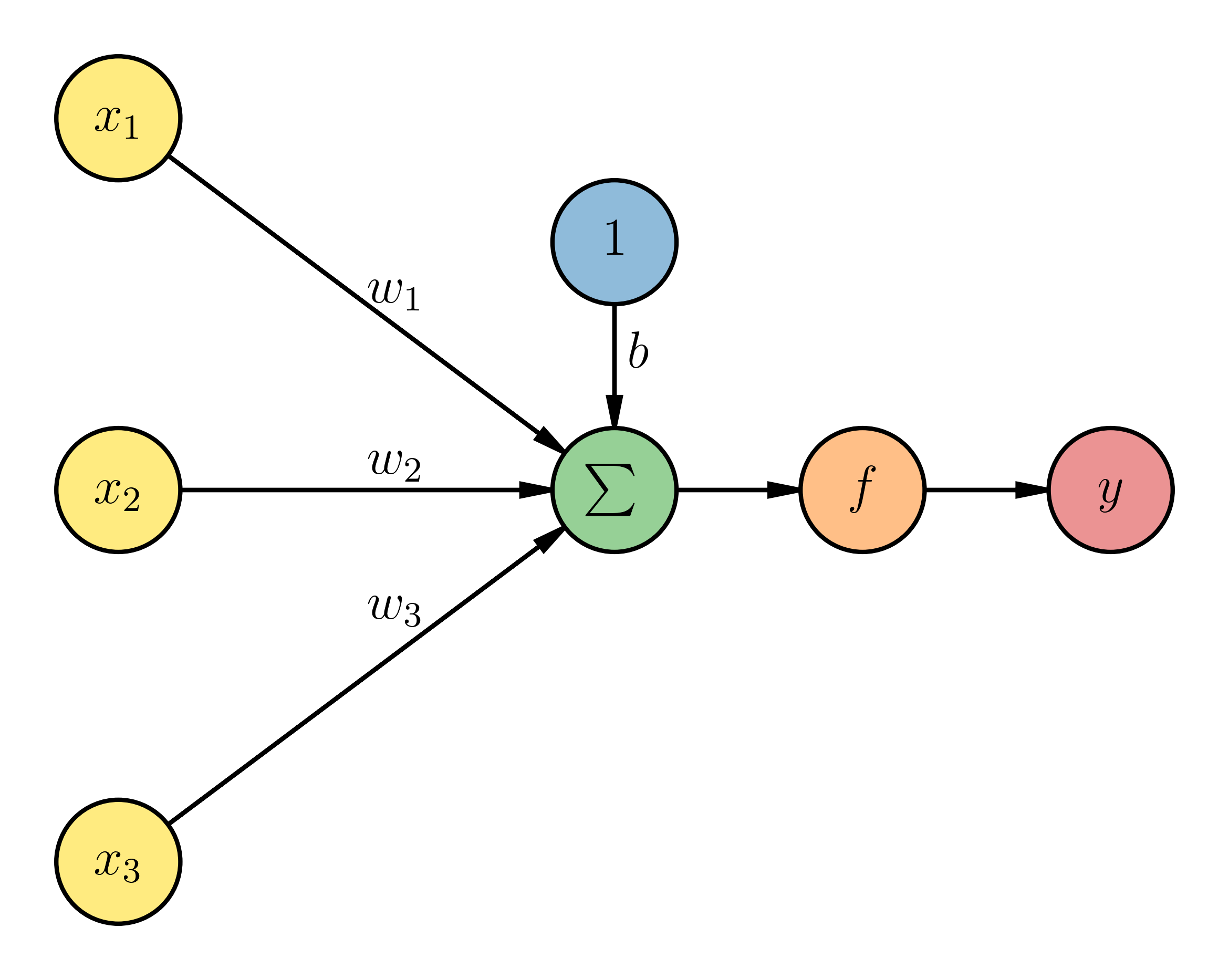
Consider what happens to the inputs of this neuron above, before the activation function. The input values \(\vec{x}\) are those from our training set for one observation. In other words, we are showing the three properties \((x_1, x_2, x_3)\) of one observation in the training set (\(D = 3\)). Each input value has an associated weight \(\vec{w}\) that we need to determine. You can see that we are also putting in a fake input value of 1, where we label the weight of that input as \(b\). The value we are providing to the activation function \({f}\) is then

Now that we have a mathematical simplification of a single neuron, let's combine multiple neurons together into one layer of neurons. Here the term layer is used to describe the structure of how neurons are connected, and the term will come up a lot. Neurons in the same layer are typically not connected to each other. Let us consider that we have some input layer, with two inputs, and then we have five neurons in the same layer. The outputs from that layer are then fed into one neuron (in the output layer) and the output of that network is what gives us our predictions. This is what our network might look like, and this is what early neural networks looked like (back when they were called Perceptrons):
You can see now our input data are being given as inputs to multiple neurons, and each of those neurons has their own weights.
Neural network architecture
Even though each neuron can learn a non-linear mapping from the data, a three neuron network is going to be pretty simplistic for most realistic problems. For the kinds of problems we're interested in we will want to have a more extensive neural network. There are two ways you could immediately extend the existing network:
- increase the number of neurons in the same layer (go wider), and/or
- increase the number of layers (go deeper).
Even if you only increased the number of neurons in the same layer, you will find that you can create an infinitely wide single-layer neural network that will be able to learn very complex non-linearities in the data! But if you also increased the number of layers you can see that you will end up with an extremely flexible neural network! Since we are doing "machine learning" (and not "principled data analysis") and we don't care about interpretability, what is stopping us from creating a very wide (many neurons per layer) and very deep (many layers) neural network?
The first problem you will encounter will be optimisation. Even if you just have a very wide single (hidden) layer neural network, you will find this to be an optimisation nightmare if you just use naive strategies. This is because the dimensionality is high, even for a network with one hidden layer, and the problem is extremely non-convex. So you could end up in a bad valley of optimisation space. That also means that your initialisation for the weights will be extremely important. And not only is there no guarantee that you would converge to the global solution (if there is one), but there are no guarantees that you would converge to any solution!
Backpropagation
For all these reasons,
- Computers became faster.
- The backpropagation algorithm was developed.
Backpropagation
Backpropagation itself is just a clever use of the chain rule for differentiation, but it is critically important for you to understand it because there are some subtle ways where it can cause everything to fail spectacularly! If you don't understand backpropagation then you will find it much harder to debug why your neural network isn't working.
Let us imagine that we have the following dataset on properties in some city. The data that we have are:
- The number of bedrooms.
- The average price per square meter for houses in that suburb.
- The price that a particular house sold for.
We will build a neural network to try to predict house prices for other properties, just given the number of bedrooms and the average price per square meter for that suburb. Here is what the training set looks like:
| Average price per square meter |
Number of bedrooms |
Sold price |
|---|---|---|
| 2,104 | 3 | 399,900 |
| 1,600 | 3 | 329,900 |
| 2,400 | 3 | 369,000 |
| 1,416 | 2 | 232,000 |
| 3,000 | 4 | 539,900 |
| 1,985 | 4 | 299,900 |
| 1,534 | 3 | 314,900 |
| 1,427 | 3 | 198,999 |
| 1,380 | 3 | 212,000 |
| 1,494 | 3 | 242,500 |
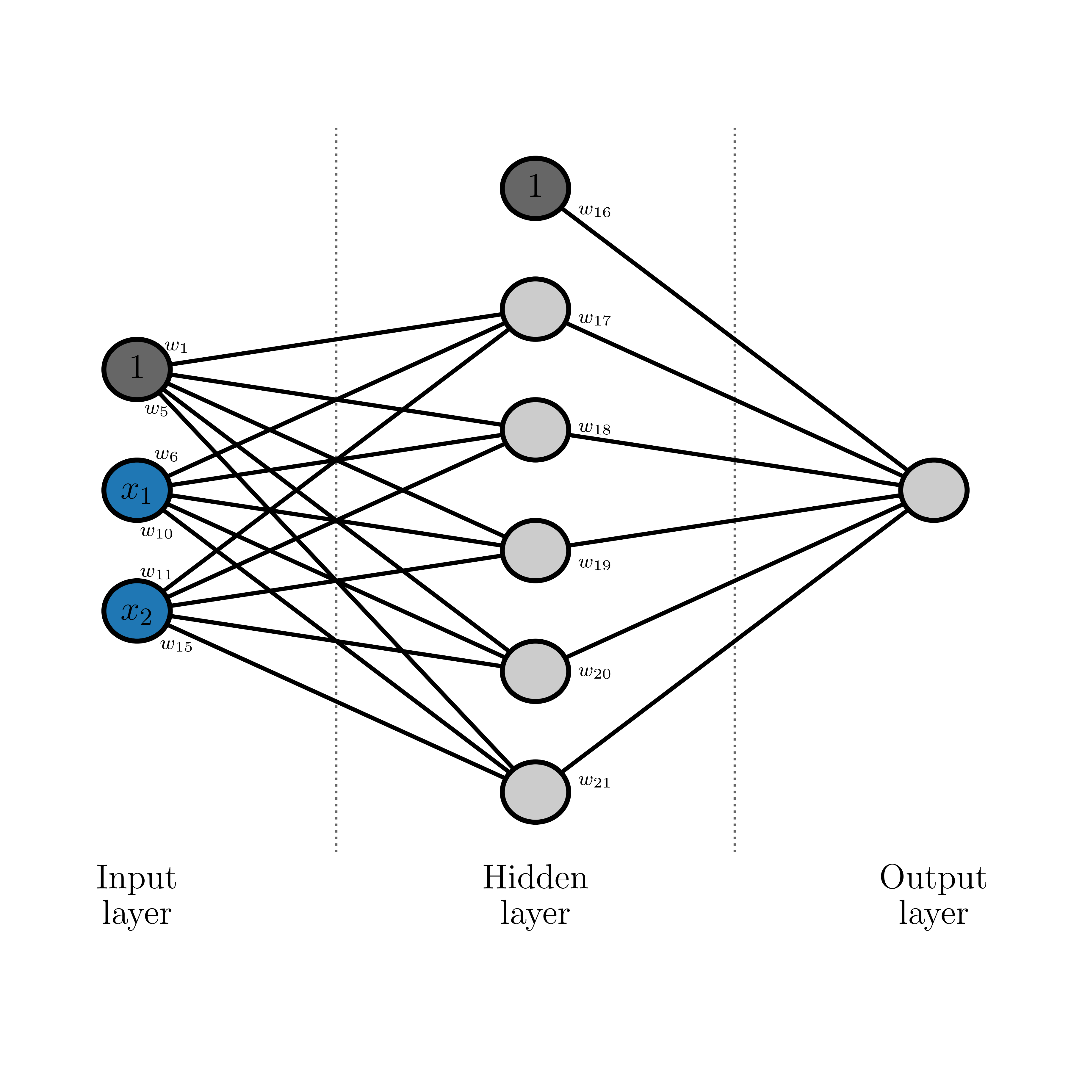
We only have ten observations. That might seem crazy because you may have heard that you need massive data sets (e.g., thousands or hundreds of thousands) to train a neural network. That's true for most situations, but we don't need a lot of data to demonstrate backpropagation. We will use the following neural network structure: 1 hidden layer with 5 neurons, and one neuron in the output layer (because there is only one thing we want to predict: house price). The structure of our network might look something like this:
Where biases are shown in grey and inputs are in blue. The weights for most edges are marked, allowing you to see how we will structure the math. Let's go through all the math before we code this up. First we will state that our original inputs are \(\vec{x^\ast}\) and \(\vec{y^\ast}\), and for good reasons that we will explain later, we will normalise these so that they have zero mean and unit variance. We will refer to the normalised inputs and outputs as \(\vec{x}\) and \(\vec{y}\). We will name neurons by their layer and their order from top to bottom: H1 for the first neuron in the hidden layer (e.g., the one connected to \(w_{17}\)), and O1 for the single output layer. We will also define the input to the activation function \(f\) of a node by \(\alpha\) (e.g., \(\alpha_{H1}\) for the net input to neuron H1) and we will define the output of the activation function of a neuron to be \(\beta\) (e.g., \(\beta_{H1} = f(\alpha_{H1})\)).
The inputs and outputs for each neuron in the hidden layer are: \[ \begin{eqnarray} \alpha_{H1} &=& w_1 + x_{1}w_{6} + x_{2}w_{11} \\ \beta_{H1} &=& f(\alpha_{H1}) \end{eqnarray} \] \[ \begin{eqnarray} \alpha_{H2} &=& w_2 + x_{1}w_{7} + x_{2}w_{12} \\ \beta_{H2} &=& f(\alpha_{H2}) \end{eqnarray} \] \[ \begin{eqnarray} \alpha_{H3} &=& w_3 + x_{1}w_{8} + x_{2}w_{13} \\ \beta_{H3} &=& f(\alpha_{H3}) \end{eqnarray} \] \[ \begin{eqnarray} \alpha_{H4} &=& w_4 + x_{1}w_{9} + x_{2}w_{14} \\ \beta_{H4} &=& f(\alpha_{H4}) \end{eqnarray} \] \[ \begin{eqnarray} \alpha_{H5} &=& w_5 + x_{1}w_{10} + x_{2}w_{15} \\ \beta_{H5} &=& f(\alpha_{H5}) \end{eqnarray} \]
And for the output layer: \[ \begin{eqnarray} \alpha_{O1} &=& w_{16} + \beta_{H1}w_{17} + \beta_{H2}w_{18} + \beta_{H3}w_{19} + \beta_{H4}w_{20} + \beta_{H5}w_{21}\\ \beta_{O1} &=& f(\alpha_{O1}) \end{eqnarray} \] where \(\beta_{O1}\) is also known as \(\vec{y}_\textrm{pred}\).
We will initialise the weights randomly. In reality we often do initialise the weights of a neural network randomly, but we don't do so uniformly — we normally want to draw from some distribution and clip values within ranges. You will learn more about that this week. For now let us assume that we have initialised the weights in The Right Way™. First let's code up our neural network. Later on you will see how to do this in PyTorch (by Facebook™) and TensorFlow (by Google™), but to get us started we will code everything in numpy.
Here we have initialised our weights randomly and completed our first forward pass through the network, where we are using the inputs and the randomised weights to make predictions \(\vec{y}_\textrm{pred}\) for house prices. These initial predictions will not be very good because our weights were randomly chosen. Indeed, the initial loss \(E\) \[ E = \frac{1}{2}\sum_{i}^{N}(y_i - y_{\textrm{pred},i})^2 \] is 6, which is a lot given that we have 10 observations that are all zero mean and unit variance! But this does show that we can feed inputs into a neural network and get it to provide us with an output! Now let's explore how we can use backpropagation to improve the weights, and improve our predictions.
The idea of backprop is to propagate the errors in our predictions back through the network and to iteratively improve the weights. Recall that in Stochastic Gradient Descent we use the derivative of the outputs with respect to the parameters to improve our estimates of those parameters. We are going to do the exact same thing here. First let's consider that we are going to update our estimate of \(w_{16}\). To do so we will need the gradient of the loss with respect to \(w_{16}\) \[ \frac{\partial{}E}{\partial{}w_{16}} \] which we know from the chain rule is \[ \frac{\partial{}E}{\partial{}w_{16}} = \frac{\partial{}E}{\partial{}\beta_{O1}} \frac{\partial{}\beta_{O1}}{\partial{}\alpha_{O1}} \frac{\partial{}\alpha_{O1}}{\partial{}w_{16}} \] where we will have to calculate each term. First let us recall that since \(y_{\textrm{pred},i} \equiv \beta_{O1,i}\), \[ E = \frac{1}{2}\sum_{i=1}^{N}\left(y_i - \beta_{O1,i}\right)^2 \] so \[ \frac{\partial{}E}{\partial{}\beta_{O1}} = -\left(y - \beta_{O1}\right) \quad . \] For the next term recall that \[ \beta_{O1} = f(\alpha_{O1}) \] where \(f\) is a sigmoid \[ \beta_{O1} = f(\alpha_{O1}) = \frac{1}{1 + e^{-\alpha_{O1}}} \] such that \[ \frac{\partial{}\beta_{O1}}{\partial{}\alpha_{O1}} = \beta_{O1}\left(1 - \beta_{O1}\right) \quad . \] And finally, \[ \alpha_{O1} = w_{16} + \beta_{H1}w_{17} + \beta_{H2}w_{18} + \beta_{H3}w_{19} + \beta_{H4}w_{20} + \beta_{H5}w_{21} \] such that \[ \frac{\partial{}\alpha_{O1}}{\partial{}w_{16}} = 1 \quad . \]
Bringing these terms together, \[ \begin{eqnarray} \frac{\partial{}E}{\partial{}w_{16}} &=& \frac{\partial{}E}{\partial{}\beta_{O1}} \frac{\partial{}\beta_{O1}}{\partial{}\alpha_{O1}} \frac{\partial{}\alpha_{O1}}{\partial{}w_{16}} \\ \frac{\partial{}E}{\partial{}w_{16}} &=& \beta_{O1}(\beta_{O1}-y)(1-\beta_{O1}) \end{eqnarray} \] allows us to update our estimate of \(w_{16}\), after we adopt some learning rate \(\eta = 10^{-6}\): \[ w_{16}^{(t+1)} = w_{16}^{(t)} - \eta\frac{\partial{}E}{\partial{}w_{16}} \quad. \] But we don't want to update one weight at a time; we want to calculate the updated weights (during the backward pass) and then update them all at once before making another prediction. Let us consider that we carefully calculated all gradients that we needed for all the weights \(w_{16}\) to \(w_{21}\), and now we are at the stage of calculating the updated weights \(w_{1}\) to \(w_{15}\). For \(w_1\) the procedure is very similar: we flow gradients back through the graph such that \[ \frac{\partial{}E}{\partial{}w_{1}} = \frac{\partial{}E}{\partial{}\beta_{O1}} \frac{\partial{}\beta_{O1}}{\partial{}\alpha_{O1}} \frac{\partial{}\alpha_{O1}}{\partial{}\beta_{H1}} \frac{\partial{}\beta_{H1}}{\partial{}\alpha_{H1}} \frac{\partial{}\alpha_{H1}}{\partial{}w_{1}} \] where we already have \[ \begin{eqnarray} \frac{\partial{}E}{\partial{}\beta_{O1}} &=& -\left(y - \beta_{O1}\right) \\ \frac{\partial{}\beta_{O1}}{\partial{}\alpha_{O1}} &=& \beta_{O1}\left(1 - \beta_{O1}\right) \end{eqnarray} \] and for \(\frac{\partial{}\alpha_{O1}}{\partial{}\beta_{H1}}\), \[ \alpha_{O1} = w_{16} + \beta_{H1}w_{17} + \beta_{H2}w_{18} + \beta_{H3}w_{19} + \beta_{H4}w_{20} + \beta_{H5}w_{21} \] such that \[ \frac{\partial{}\alpha_{O1}}{\partial{}\beta_{H1}} = w_{17} \] and just like \(\frac{\partial{}\beta_{O1}}{\partial{}\alpha_{O1}}\), \[ \frac{\partial{}\beta_{H1}}{\partial{}\alpha_{H1}} = \beta_{H1}\left(1 - \beta_{H1}\right) \] which leads to the final term \(\frac{\partial{}\alpha_{H1}}{\partial{}w_{1}}\) where \[ \alpha_{H1} = w_1 + x_{1}w_{6} + x_{2}w_{11} \] such that \[ \frac{\partial{}\alpha_{H1}}{\partial{}w_{1}} = 1 \quad . \] Bringing it all together yields \[ \begin{eqnarray} \frac{\partial{}E}{\partial{}w_{1}} &=& \frac{\partial{}E}{\partial{}\beta_{O1}} \frac{\partial{}\beta_{O1}}{\partial{}\alpha_{O1}} \frac{\partial{}\alpha_{O1}}{\partial{}\beta_{H1}} \frac{\partial{}\beta_{H1}}{\partial{}\alpha_{H1}} \frac{\partial{}\alpha_{H1}}{\partial{}w_{1}} \\ \frac{\partial{}E}{\partial{}w_{1}} &=& \left(\beta_{O1} - y\right)\beta_{O1}\left(1 - \beta_{O1}\right)w_{17}\beta_{H1}\left(1 - \beta_{H1}\right) \end{eqnarray} \] such that the updated estimate for \(w_1^{(t+1)}\) is \[ w_1^{(t+1)} = w_1^{(t)} - \eta\frac{\partial{}E}{\partial{}w_{1}} \quad . \] And you can see that this process can be repeated (and needs to be) for all weight terms. In doing so you should find: \[ \begin{eqnarray} \frac{\partial{}E}{\partial{}w_{1}} &=& \left(\beta_{O1} - y\right)\beta_{O1}\left(1 - \beta_{O1}\right)w_{17}\beta_{H1}\left(1 - \beta_{H1}\right) \\ \frac{\partial{}E}{\partial{}w_{2}} &=& \left(\beta_{O1} - y\right)\beta_{O1}\left(1 - \beta_{O1}\right)w_{18}\beta_{H2}\left(1 - \beta_{H2}\right) \\ \frac{\partial{}E}{\partial{}w_{3}} &=& \left(\beta_{O1} - y\right)\beta_{O1}\left(1 - \beta_{O1}\right)w_{19}\beta_{H3}\left(1 - \beta_{H3}\right) \\ \frac{\partial{}E}{\partial{}w_{4}} &=& \left(\beta_{O1} - y\right)\beta_{O1}\left(1 - \beta_{O1}\right)w_{20}\beta_{H4}\left(1 - \beta_{H4}\right) \\ \frac{\partial{}E}{\partial{}w_{5}} &=& \left(\beta_{O1} - y\right)\beta_{O1}\left(1 - \beta_{O1}\right)w_{21}\beta_{H5}\left(1 - \beta_{H5}\right) \\ \frac{\partial{}E}{\partial{}w_{6}} &=& \left(\beta_{O1} - y\right)\beta_{O1}\left(1 - \beta_{O1}\right)w_{17}\beta_{H1}\left(1 - \beta_{H1}\right)x_1 \\ \frac{\partial{}E}{\partial{}w_{7}} &=& \left(\beta_{O1} - y\right)\beta_{O1}\left(1 - \beta_{O1}\right)w_{18}\beta_{H2}\left(1 - \beta_{H2}\right)x_1 \\ \frac{\partial{}E}{\partial{}w_{8}} &=& \left(\beta_{O1} - y\right)\beta_{O1}\left(1 - \beta_{O1}\right)w_{19}\beta_{H3}\left(1 - \beta_{H3}\right)x_1 \\ \frac{\partial{}E}{\partial{}w_{9}} &=& \left(\beta_{O1} - y\right)\beta_{O1}\left(1 - \beta_{O1}\right)w_{20}\beta_{H4}\left(1 - \beta_{H4}\right)x_1 \\ \frac{\partial{}E}{\partial{}w_{10}} &=& \left(\beta_{O1} - y\right)\beta_{O1}\left(1 - \beta_{O1}\right)w_{21}\beta_{H5}\left(1 - \beta_{H5}\right)x_1 \\ \frac{\partial{}E}{\partial{}w_{11}} &=& \left(\beta_{O1} - y\right)\beta_{O1}\left(1 - \beta_{O1}\right)w_{17}\beta_{H1}\left(1 - \beta_{H1}\right)x_2 \\ \frac{\partial{}E}{\partial{}w_{12}} &=& \left(\beta_{O1} - y\right)\beta_{O1}\left(1 - \beta_{O1}\right)w_{18}\beta_{H2}\left(1 - \beta_{H2}\right)x_2 \\ \frac{\partial{}E}{\partial{}w_{13}} &=& \left(\beta_{O1} - y\right)\beta_{O1}\left(1 - \beta_{O1}\right)w_{19}\beta_{H3}\left(1 - \beta_{H3}\right)x_2 \\ \frac{\partial{}E}{\partial{}w_{14}} &=& \left(\beta_{O1} - y\right)\beta_{O1}\left(1 - \beta_{O1}\right)w_{20}\beta_{H4}\left(1 - \beta_{H4}\right)x_2 \\ \frac{\partial{}E}{\partial{}w_{15}} &=& \left(\beta_{O1} - y\right)\beta_{O1}\left(1 - \beta_{O1}\right)w_{21}\beta_{H5}\left(1 - \beta_{H5}\right)x_2 \\ \frac{\partial{}E}{\partial{}w_{16}} &=& \left(\beta_{O1} - y\right)\beta_{O1}\left(1 - \beta_{O1}\right) \\ \frac{\partial{}E}{\partial{}w_{17}} &=& \left(\beta_{O1} - y\right)\beta_{O1}\left(1 - \beta_{O1}\right)\beta_{H1} \\ \frac{\partial{}E}{\partial{}w_{18}} &=& \left(\beta_{O1} - y\right)\beta_{O1}\left(1 - \beta_{O1}\right)\beta_{H2} \\ \frac{\partial{}E}{\partial{}w_{19}} &=& \left(\beta_{O1} - y\right)\beta_{O1}\left(1 - \beta_{O1}\right)\beta_{H3} \\ \frac{\partial{}E}{\partial{}w_{20}} &=& \left(\beta_{O1} - y\right)\beta_{O1}\left(1 - \beta_{O1}\right)\beta_{H4} \\ \frac{\partial{}E}{\partial{}w_{21}} &=& \left(\beta_{O1} - y\right)\beta_{O1}\left(1 - \beta_{O1}\right)\beta_{H5} \end{eqnarray} \]
Let's code this up.
Before we run this, let's have a brief aside on why (and how!) you should check your derivatives when coding something like this up.
Check your derivatives!
Whenever you are coding up something that involves derivatives you should follow these rules:
- Don't calculate them yourself unless you have to. (Let a computer do it for you!)
- If you have to calculate them yourself, check it numerically!
Let's check our derivatives numerically:
If all goes well,..
Then after we run our neural network then we should see the loss reducing with time. Let's see:

Nice! But is that it? Do we really have to code every neural network ourselves and calculate all those derivatives? Of course not. Once you understand something well enough to code it up yourself, you should use a package that is well-engineered for performance. Here is the equivalent code in PyTorch:
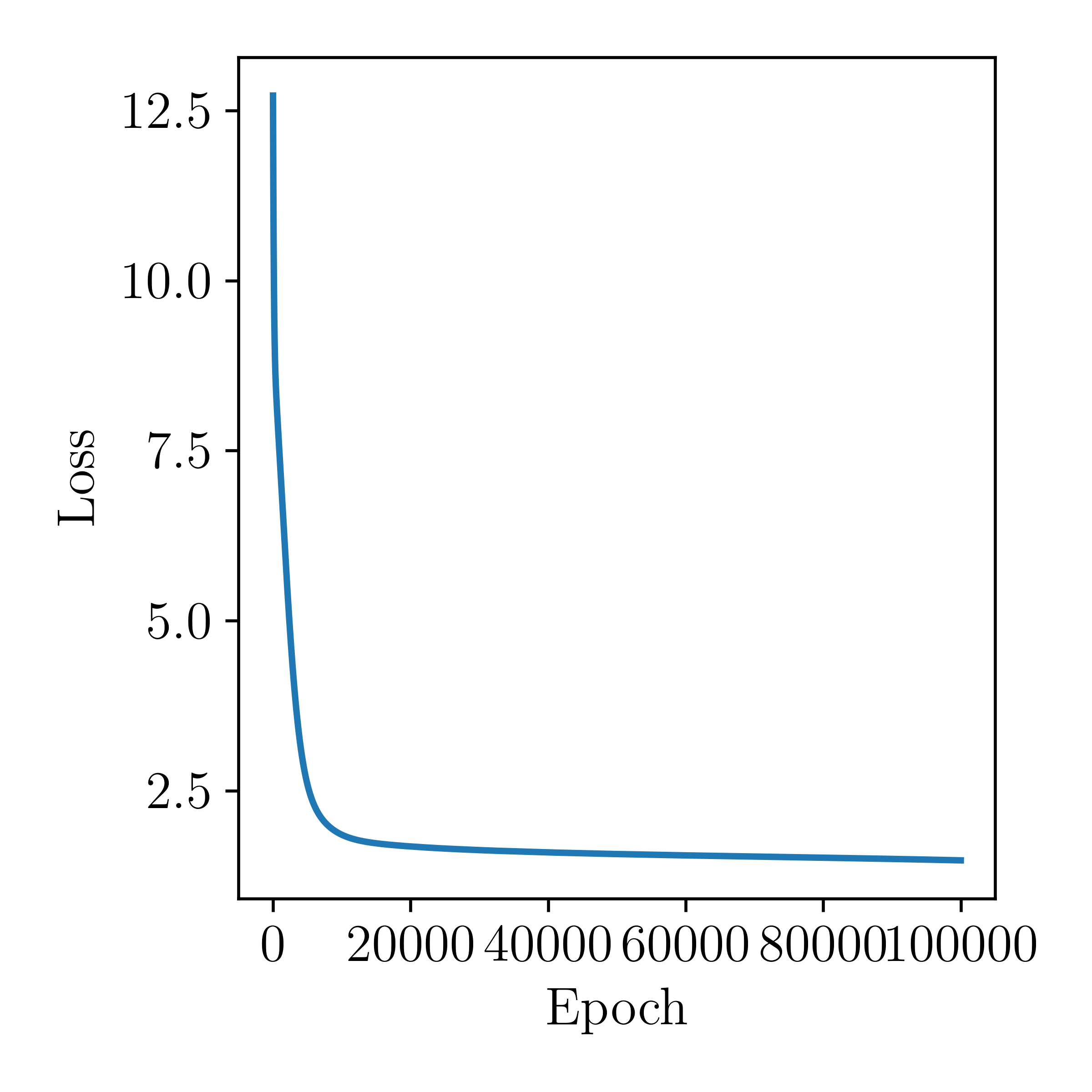
Let's plot the loss as a function of epoch for this model:
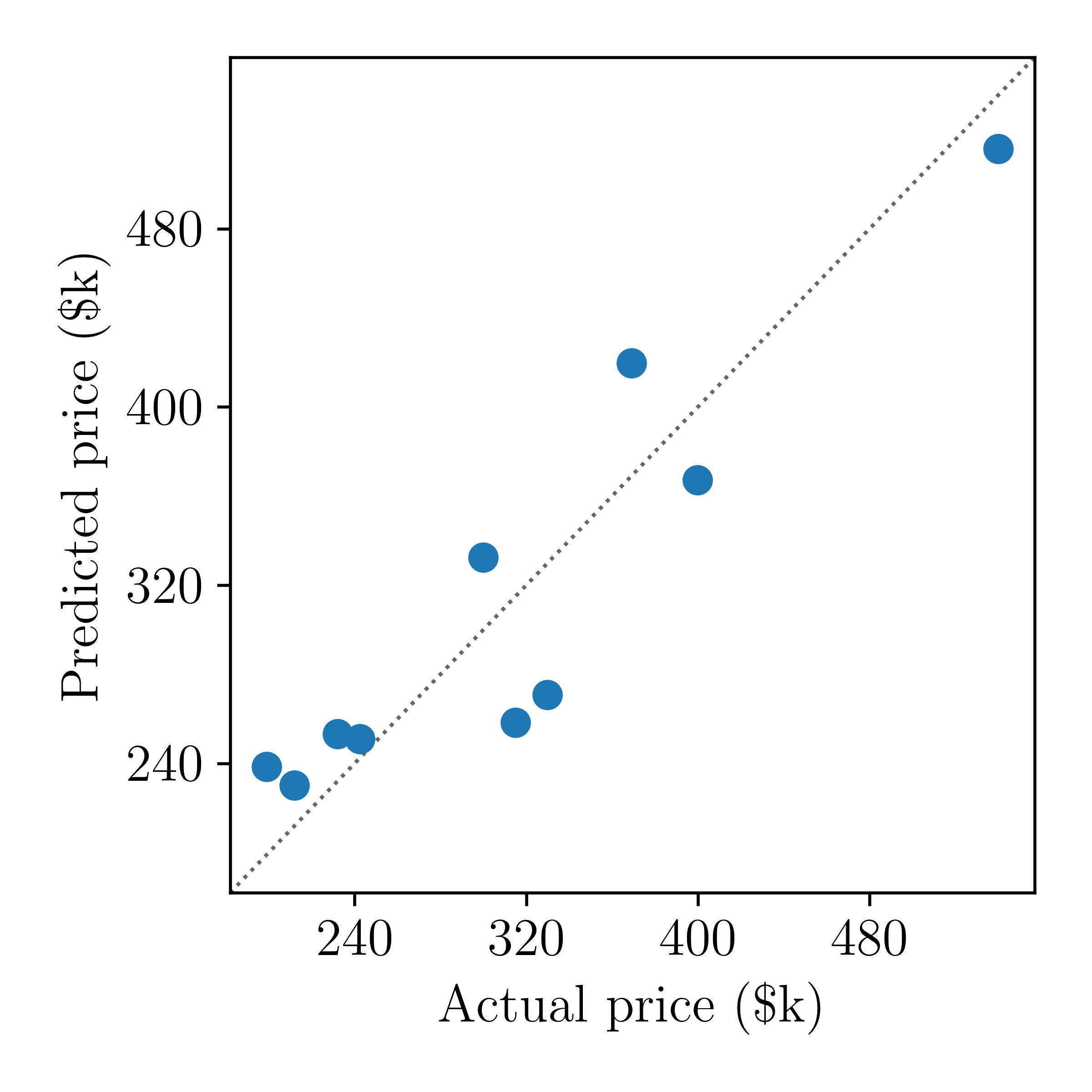
Much nicer! Now let's look at the actual predictions from the model, compared to the actual prices.
Looks good! But why was the loss curve so different for our numpy implementation than that of the PyTorch model? There are many reasons for this, which — now that you know how backpropagation works — we will go through.
Backpropagation problems
Vanishing gradients
In our network we are using sigmoids as the activation function. That's fine, but let's consider what happens if we were to initialise the weights incorrectly, or if we didn't scale the initial data set properly. If our weights are too large then the net input \(\alpha\) into the sigmoid function \(f\) is going to be larege, which means the output \(\beta\) is going to be near 1. In theory that is OK: the neuron has been activated. But consider the backpropagation step! The derivative of a sigmoid \[ \beta = f(\alpha) = \frac{1}{1 + e^{-\alpha}} \] is \[ \frac{\partial\beta}{\partial\alpha} = \beta(1-\beta) \quad . \] If the net input \(\alpha\) is too high then the output \(\beta\) will be 1, which means that the derivative over that neuron will be zero! And depending on where that neuron is in the network, that could mean that many of our gradients end up vanishing to zero because those gradients get multiplied by zero. So we could lose many gradients simply because one neuron had a set of weights being too high! And because the gradient is zero, there will be no updates to the relevant weights. That means vanishing gradients like this — caused by either bad initialisation, noisy optimisation, or incorrectly scaled data set — can totally kill a large part of your network! So if you're using sigmoids (or tanh functions) then you should worry about saturating them.
Dead neurons
This is a different, but related problem. Let's introduce you to another activation function: the Rectified Linear Unit (ReLU) function. The function is defined by
\[
f(x) = \textrm{max}(0, x)
\]
and has an activation profile as:
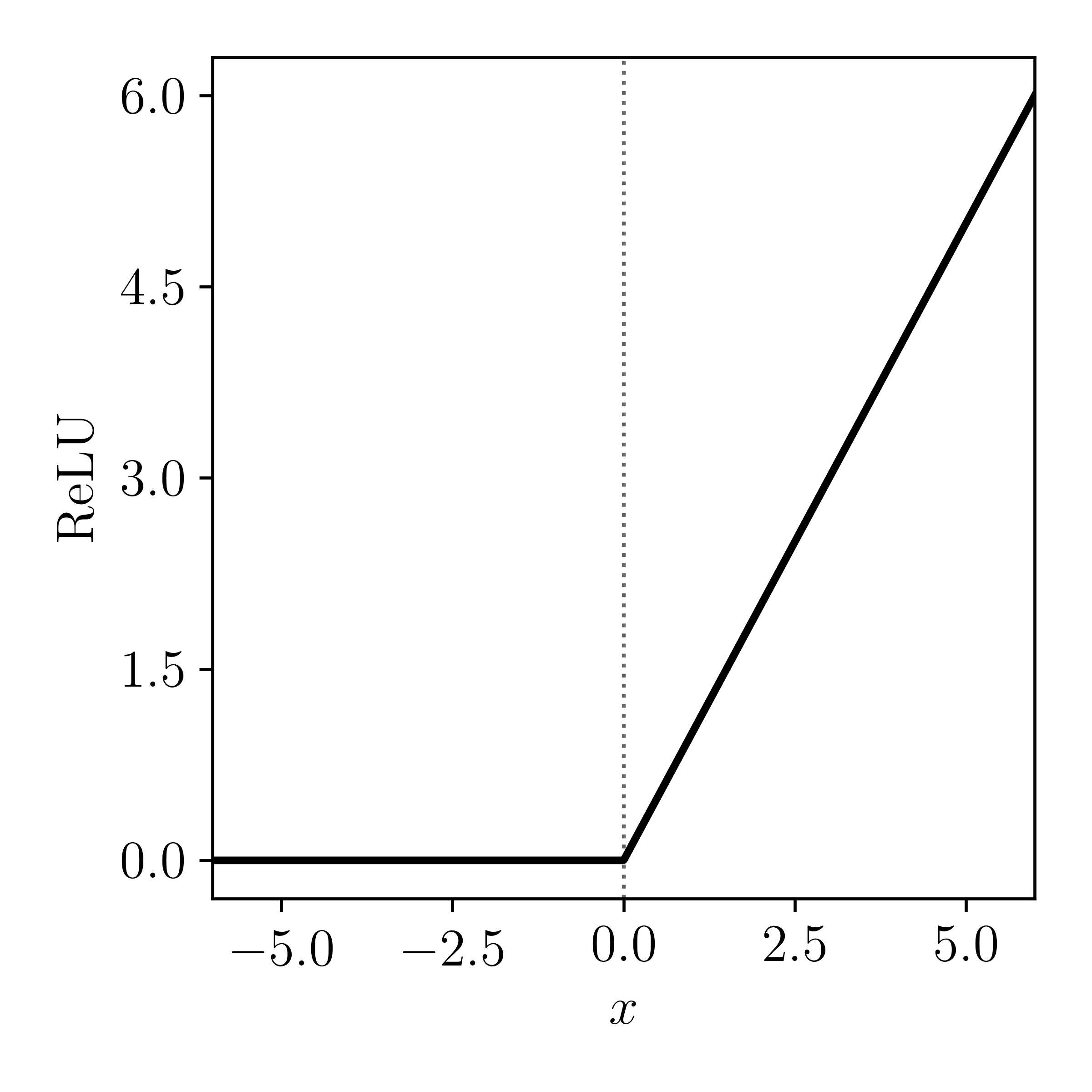
That means if the input value is less than zero then the neuron won't fire. And if the input value gets very low, the gradient vanishes away to zero. When that happens you effectively have the same problem as a saturated sigmoid function: one of your neurons is permanently dead and it will cause all other neurons in the same multiplicative chain to be zero as well. This can happen through bad initialisation, or through an update step during training if the learning rate was too high.
Explosive gradients
Hopefully you're starting to get the picture that gradients across one neuron can have a flow-on effect in the rest of the network. But zero-ing out neurons is not the only problem. In Recurrent Neural Networks (RNNs; which we will cover next week) you can have neurons that are fed information between states for many time steps. When that happens it is the same as if you have some small error that builds up over time. It's the same as taking the multiplication between two numbers \(a\) and \(b\) like \(abbbbbbbb\)... If \(|b| > 1\) then the network will eventually go to infinity, and if \(|b| < 1\) then the network will eventually go to zero. In either case, you are going to have a bad time!
Noisy updates and aggressive learning rates
Often when you train a neural network you won't want to use all of the data to update the weights. Instead you might decide to use a single observation, or a small batch of data, to update the weights. When that happens you are doing fewer calculations and approximating the gradient of the entire data set. If you are using a learning rate that is too high, then the error introduced by this approximate gradient can cause the weights to be updated too much (or too little), and send your neural network into a spiraling mess. If this happens you will see your loss function accelerating up with increasing epochs.
Summary
Neural networks are a simplified mathematical description of how we think humans think. Although they are a significant simplification of how a neuron actually works, they are sufficiently flexible that they are often referred to as universal interpolators because they can learn any non-linear relationship from data. There are many choices you have to face when designing a neural network, including the structure of the network, initialisation, optimisation, activation functions, et cetera. Even if you get all those choices correct, it can still be difficult to train a neural network! Backpropagation was the key step that allowed us to train complex neural networks, but backpropagation will not solve all your problems! You must think carefully about how backpropagation will be executed on your network in order to understand how it will fail.
In the next class we are going to cover how to train neural networks in practice. This will include how to chose between activation functions, how to initialise your weights correctly, how to prepare your data correctly for neural networks, and things like dropout. After that we will go through neural network architecture design.