Today we will go through a few different key dimensionality reduction algorithms, and we will speak a little bit about matrix factorisation methods. Matrix factorisation methods are a — sort of — dimensionality reduction in that you may be trying to take a huge matrix of shows that people have watched on Netflix™ and you are wanting to find an embedding that makes sensible predictions for other users. These kinds of recommendation systems are probably better described by some kind of latent variable model, but for lack of better organisation we will discuss them briefly today!
Dimensionality reduction
Dimensionality reduction is the statistical procedure of reducing the dimensionality of some data set, while preserving much of the statistical representation of the original data set. Dimensionality reduction falls into the category of unsupervised machine learning algorithms because they do not require an explicit labelled set from an expert (human). Dimensionality reduction techniques often form part of a machine learning workflow because we are usually interested in having some lower-dimensional interpretation for the data, but it is not usually the final thing we are interested in.
Principal Component Analysis
Principal Component Analysis (PCA) is the simplest and most well-known dimensionality reduction technique. PCA is a method of reducing (potentially correlated) variables into a set of orthogonal and linearly independent vectors, which we call principal components. The first principal component is the vector along which most of the data exist, and the second principal component will be orthogonal to that first vector. Drag the data points around in the following visualisation to see how the principal coordinate system adjusts, and how the data points can be represented in their original data space (left) or in the principal component coordinate system (right).
Here we are only using PCA to change the coordinate system, but we can also use PCA to reduce the dimensionality of the data. Take a look at this cloud of points in three dimensions as it rotates about some \(x\), \(y\), \(z\) axes. You can see the projection of these data in the centre panel, where you are looking at a two-dimensional projection along the blue axes. Now use the centre panel to vary the camera projection. While varying the camera projection, look at the data points along each principal component in the bottom right hand side. Try to align the camera projection such that most of the variance is contained along the first principal component, \(\textrm{pc}1\), and then the second component has the next most amount of variance, and \(\textrm{pc}3\) has the least variance. If you do that correctly then when you push the Show PCA button the projection should not change much!
How does this help with dimensionality reduction? Well you can see that when you aligned the camera projection
PCA is about finding an orthogonal projection that best describes the variance in the data, and then either using those principal components to explore relationships in the data,
PCA has many similarities to other matrix factorisation techniques, including singular value decomposition. Let us assume we have a mean-centered data matrix \(\vec{X}\) such that the mean of each column has been subtracted off, leaving a mean of zero in each dimension. We will assume that there are \(N\) measurements and each measurement has \(D\) dimensions, such that \(\vec{X}\) has shape \(N\times{}D\).
We can compute the \(D \times{} D\) covariance matrix \(\vec{C}\) of the data \(\vec{X}\) by taking \[ \vec{C} = \frac{1}{N-1}\vec{X}\transpose\vec{X} \quad . \] Since \(\vec{C}\) is a covariance matrix, and all covariance matrices are symmetric, it can be diagonalised \[ \vec{C} = \vec{VLV}\transpose \] where \(\vec{V}\) is a matrix of eigenvectors where each column is an eigenvector, and \(\vec{L}\) is a diagonal matrix with eigenvalues \(\lambda_i\) in decreasing order along the diagonal. The eigenvectors are the same thing as the principal axes or principal directions of the data. Since the eigenvalues are in decreasing order, the first column of \(\vec{V}\) is the first principal component.
To project the data on \(\vec{X}\) along the principal axes — or rather, along the eigenvectors — we calculate \(\vec{XV}\) and we call these the principal component scores. The \(j\)-th principal component is given by the \(j\)-th column of \(\vec{XV}\). The coordinates of the \(i\)-th data point in the new principal component space are given by the \(i\)-th row of \(\vec{XV}\).
If you're familiar with singular value decomposition \[ \vec{X} = \vec{USV}\transpose \] then you will appreciate that \[ \begin{eqnarray} \vec{C} &=& \frac{1}{N-1}\vec{VSU}\transpose\vec{USV} \\ \vec{C} &=& \frac{1}{N-1}\vec{VS}(\vec{U}\transpose\vec{U})\vec{SV} \\ \vec{C} &=& \frac{1}{N-1}\vec{VSISV} \\ \vec{C} &=& \vec{V}\frac{\vec{S}^2}{N-1}\vec{V}\transpose \end{eqnarray} \] meaning that the vectors in \(\vec{V}\) from singular value decomposition are principal directions and \(\vec{L} = \frac{\vec{S}^2}{N-1}\) contains the eigenvalues such that \(\lambda_i = s_i^2/(N-1)\). If we substitute \(\vec{X} = \vec{USV}\transpose\) when calculating principal component projections \(\vec{XV}\) this becomes \[ \begin{eqnarray} \vec{XV} &=& (\vec{USV}\transpose)\vec{V} \\ \vec{XV} &=& \vec{USV}\transpose\vec{V} \\ \vec{XV} &=& \vec{US} \quad . \end{eqnarray} \]
If you instead wanted to do things by hand you could calculate the eigenvalues \(\lambda\) by calculating \[ \vec{C} = \frac{1}{N-1}\vec{X}\transpose\vec{X} \] then remembering that the eigenvalues are roots of the characteristic equation \(\det(\vec{C} - \lambda\vec{I}) = 0\), and then calculate the corresponding eigenvectors for those eigenvalues.
PCA has many uses in physics and astronomy.
t-distributed Stochastic Neighbour Embedding
If you have ever used t-distributed Stochastic Neighbour Embedding (t-SNE) before then you may have thought it was magic.
2. Stop letting other people think that.
Unlike PCA, t-SNE does not take linear projections of the data. It uses local relationships (like correlations) between points to create a low-dimensional mapping. Just like Gaussian Processes and the kernel trick, this allows t-SNE to capture non-linear structure — which standard PCA cannot!
Let's look at how it works. We will spare the technical implementation details and focus on the algorithmic ones.
Step 1: Define a probability distribution over neighbours
We need to define a probability distribution over neighbours in data space.
- Pick one point in the dataset \(x_i\).
- Define the probability of picking another point \(x_j\) in the dataset as the neighbour as \[ p_{ji} = \frac{\exp\left(-\frac{\lVert{}x_i-x_j\rVert{}^2}{2\sigma_i^2}\right)}{\sum_{k\neq i} \exp\left(-\frac{\lVert{}x_i-x_k\rVert{}^2}{2\sigma_i^2}\right)} \] where we have yet to define \(\sigma_i\).
This states that the probability of picking \(x_j\) as the neighbour for \(x_i\) is a Gaussian centered on \(x_i\). For \(\sigma_i\), we want this value to be small for points in densely populated areas of data space, and to be large for sparesly populated areas in data space. The reason for this is because in the t-SNE projection we want the number of neighbours to be roughly the same for all points to prevent any single pointing from showing disproportionate influence. So the way we quantify this is by introducing a hyperparameter called the perplexity, which is basically the effective number of neighbours for any point. Larger perplexities will take more global structure into account, and smaller perplexities will make embeddings more locally focussed.
Step 2: Recreate the probability distribution in projected space
Let us express the low-dimensional mapping of the data point \(x_i\) as \(y_i\). Intuitively we want the low-dimensional mappings to express a similar probability distribution as the higher-dimensional probability distribution in Step 1. But if we directly use a Gaussian distribution then we will still end up with a crowding problem, where single data points will tend to dominate. Instead we want to use a probability distribution that has a longer tail to it. For this reason, t-SNE uses a Cauchy distribution — also known as the t-student distribution. This (joint) probability density between points \(y_i\) and \(y_j\) is \[ q_{ji} = \frac{\left(1 + \lVert{}y_i - y_j\rVert{}^2\right)^{-1}}{\sum_{k \neq l}\left(1 + \lVert{}y_k - y_l\rVert{}^2\right)^{-1}} \quad . \]
t-SNE seeks for these two probabilities \(p_{ji}\) and \(q_{ji}\) to be as similar as possible, over all points. This is achieved using gradient descent on the Kullback-Liebler divergence from the distribution \(p\) to \(q\). This needs to be calculated across all points, which immediately gives you an idea for how poorly t-SNE scales with larger data sets. It should also give you some idea for how non-convex this problem is, and how non-deterministic t-SNE is: you can run t-SNE multiple times and get a different result each time!
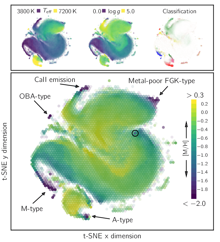
But people like t-SNE because it makes pretty pictures, that often the analyst can try to explain representations as being causal explanations. But most people are unaware of how counter-intuitively the perplexity hyperparameter can influence their results, and they don't appreciate that these are just linear embeddings. With the 'wrong' perplexity value you can
- see clustering in data when there is none, and
- find no clustering in data when there clearly is.
In other words: t-SNE can fail very quietly, in very subtle ways, and the output depends on your random seed! Don't believe any science that people show you with t-SNE unless they can describe a generative model
Finally, unlike PCA, t-SNE does not define a function to reduce dimensionality. That means you can't use t-SNE to compress data, only to visualise a lower-dimensional projection of some large data set. If you are still interested in using t-SNE but can't afford to — because you have data set sizes from The Real World™ — then you may be interested in UMAP. And if you're still interested in dimensionality reduction techniques, check out:
- Kernel PCA
- Linear discriminant analysis
- Autoencoders, which we will revisit in later weeks!
Matrix factorisation; recommender systems
Imagine if you owned Netflix and you had a large matrix of ratings where users have watched a movie and given a ranking between one and five stars. This matrix will obviously be sparse, in that not all users would have watched all movies. In fact, it will likely be very sparse in that most elements of this matrix will probably be empty!
You would like to produce a recommendation system users, in order to recommend which kind of movies they might want to watch. It turns out that matrix factorisation is a very reasonable approach for a problem like this! Consider that the matrix of ratings that you have is actually constructed from two lower dimensional matrices, one that has entries for individual users, and another with entries for movies.
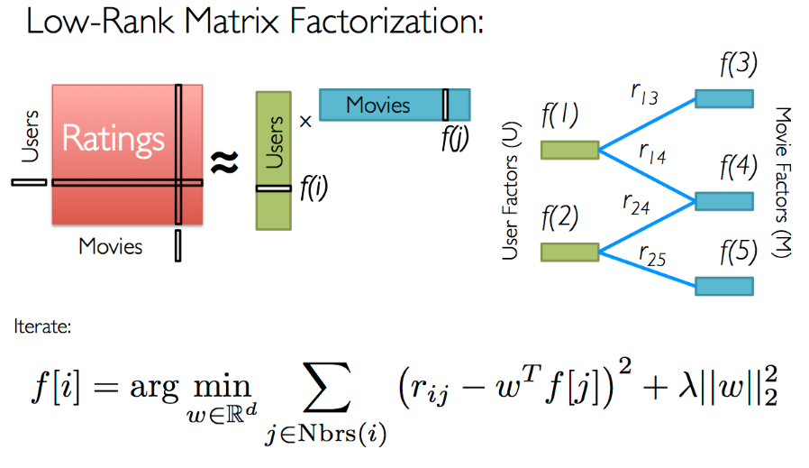
In theory this would be very similar to singular value decomposition, but in practice we can't use SVD here because our matrices are extremely sparse. Instead we will write the entries of the ratings matrix \(\vec{r}\) to be \[ r_{ui} = q_{i}\transpose{}p_{u} \] where \(\vec{q}\) is a \(M\times{}K\) matrix of (latent) user attributes, and \(\vec{p}\) is a \(K\times{}N\) matrix. Since the rating matrix is sparse we can write this as an optimisation problem where our objective function is \[ \min_{q,p} \sum_{(u,i)} \left(r_{ui} - q_{i}\transpose{}p_{u}\right)^2 + \lambda\lVert{}q_i\rVert{}^2 + \lambda\lVert{}p_u\rVert{}^2 \quad . \] You will recognise that this is a regularised optimisation problem because we don't want to over-fit the original matrix. Otherwise we would not be able to generalise the previous ratings in a way that would accurately predict future ratings.
It is worth noting that this kind of recommendation system can also be set up in such a way where movies are grouped together in their subsets. For example, you might like Scary Cult Movies from the 1980s (a real category on Netflix), but you may have only watched one of them. Another user who has watched many of them, but not exactly the one that you had watched. If Netflix were to make predictions just based on the movies that you had watched, there would be nothing in common between the two of you. If instead, Netflix took something like the mean of ratings for each sub-category, then Netflix would predict that you might like other movies in the same category. This is an obvious prediction, but this matrix factorisation allows us to make predictions in a quantatitve way!
It is also worth stating that this kind of matrix factorisation does not necessarily require explicit results for individual users (i.e., ratings). Instead the matrix of rankings could be something like whether that user watched the movie to its completion or not, or if they tried to watch it and ended up stopping it half way through. These are implicit ratings, in a sense, that are noisier. How would you use implicit information like this to make predictions?
Summary
Dimensionality reduction methods and matrix factorisation are very useful algorithms in machine learning, and they span the regimes of unsupervised (i.e., dimensionality reduction) and supervised learning. One method that is very related to all of these topics, which we have not covered, are autoencoders. If you are interested in these topics, you should also investigate autoencoders. If you aren't interested in these topics, then I don't care, because we will revisit autoencoders in the coming weeks.
In the next class we will cover clustering techniques, and that will complete our crash course into the basics of classical machine learning techniques, before we move on to neural networks.