In this class we will start with an introduction on topics in machine learning. Many people are enticed by the idea of machine learning because they are amazed by the idea that computers can learn things and do things on their own. However, as soon as you learn about how most machine learning algorithms work you will find that they are not as special as they first appeared.The exception here is deep neural networks. There is no deep theoretical basis for how they work, why they work, or how neural networks should be structured. They are simply algorithms that are performing regression given large data sets. In other words: machine learning in of itself is nothing special, it is just statistics with a good public relations manager.

Broad categories of classical machine learning methods, from Machine Learning for Everyone.

Supervised and unsupervised learning

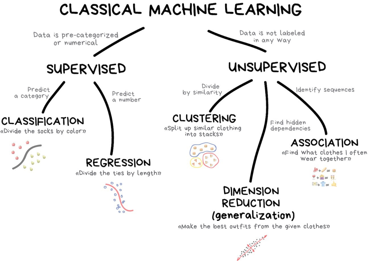
Many algorithms in machine learning can be grouped into either being a supervised machine learning algorithm, or an unsupervised algorithm. There are other relevant groupings, such as semi-supervised learning and reinforcement learning, but we will cover these in more depth in later lectures. Reinforcement learning has been a big part of many impressive advances in machine learning in recent years, including AlphaGo, self-driving cars, robotics, and video games.

Supervised learning

Supervised methods take in two kinds of training data: a set of objects for which you have input data (e.g., images, or features) and a set of associated labels for those objects. The labels for those images could be things like 'dog', 'cat', 'horse', and these are considered to be ground truths that an expertA human, usually. has provided. The labels don't have to be discrete classifications: they might also be continuous variables, like the length of a dog, it's weight, or the amount of food it eats per day.

Most machine learning algorithms fall under the category of supervised learning. That's because:

In this lecture we will cover regression and classification. We will introduce many algorithms in each of these topics to give you an idea for what algorithms are available. You should try to understand how each of these algorithms work so that you know what is appropriate given some problem, and data. In the rest of the week we will cover some unsupervised topics, including clustering, dimensionality reduction, and association.

Unsupervised learning

Unsupervised methods still take in input data, but not in the same way that supervised methods do. Supervised methods require both a set of input data (e.g., images) and associated labels. As a general rule, unsupervised methods should take in all kinds of input data (e.g., images, text, video, numerical data) and be able to draw inferences about the input data without any expert labelling. This is what most people probably naively think about when they hear 'machine learning' but in fact most machine learning methods are supervised, not unsupervised.

That means there are many advances to be made in unsupervised methods. The pioneers of neural networks individually state that the future of machine learning (and artificial intelligence) will be in developing unsupervised learning methods. This is in part because unsupervised methods should be able to make inferences from data that we did not allow for (i.e., allowing machines to be creative), and because there is so much more unlabelled data in the world than what there is labelled data. For example, there are about 300 hours worth of video uploaded to YouTube every minute. If you had an unsupervised learning method that was able to make sense of all that video as it is uploaded then you'd be unimaginably rich and famous. The problem is It's Hard™.

The most commonly used algorithms in unsupervised learning tend to be ones that involve clustering and dimensionality reduction. This is because these methods have grown naturally from the field of statistics, and they don't require any explicit labelling. This is just another way of saying that there are many advances to be made in the field of unsupervised learning!

Regression

Regression is used when you want to predict an output value, given some existing data set and an input value.

We have covered regression already. We covered it when fitting a model to data, and in hierarchical models. Here we will talk about some of the problems in regression, and the techniques used to overcome them.

Overfitting and underfitting

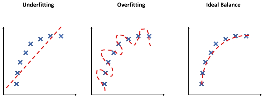
If you have some data that you want to perform polynomial regression on, but you don't know what order of polynomial you should use, then there is a tendancy to keep increasing the order of polynomial because that improves the log likelihood of the model. As you should know by now, this will result in overfitting: your model will make very bad predictions elsewhere because it has been over-fit to the data that you have. In other words, your model has overlearned a relationship in the training data to the point that it picks up patterns that are not representative in the real world.

The opposite of overfitting is, obviously, underfitting. That's where your model is not complex enough to capture the relationships in the training set. Underfitting and overfitting is closely related to the bias-variance tradeoff, an important concept in machine learning. Bias is the amount of error that is introduced by approximating the real world with a simplified model.In other words: we rarely have the true model, we are usually approximating the true model, and that approximation has error! Variance is how much your model predictions change based on variations in the training data. As a model increases in complexity (i.e., higher polynomial order) it's bias decreases because it does a good job of explaining the training data. But as the complexity increases it also becomes more wiggly (flexible), and it's variance increases (so it does not generalise to new data). Ultimately to have a good model you need one with low bias and low variance.

Visual demonstration of under-fitting, over-fitting, and ideal balance (source).

How do we address under-fitting and over-fitting?

Underfitting is often forgotten because the solution seems simple: just add more complexity to the model!In practice the method is far more subtle than this, but normally over-fitting is a bigger problem than under-fitting, so we are going to keep it simple with under-fitting.

To manage over-fitting you could decrease the order of the polynomials, or use information theory to say what maximum order is preferred, or you could use something like a Gaussian Process. In machine learning often a Gaussian Process can be too expensive for the given data set, and often you may want to include higher order terms in your polynomial model, but you just want to force the coefficients of those higher order terms to be zero unless the data really wants them to be non-zero!

Regularisation

Regularisation is often used to balance under- and over-fitting. You want a model to be sufficiently complex so that it could reasonably describe the data, but you want to place constraints on the coefficients of higher order terms so that they don't go crazy. Regularisation is the process of altering our objective function so that it forces the weight coefficients to zero, unless the data really want the coefficient to be non-zero.

Imagine a problem of the form \[ \vec{Y} = \vec{A}\vec{w} \] where \(\vec{Y}\) are the output predictions, \(\vec{A}\) is a design matrix of features, and \(\vec{x}\) is a vector of unknown coefficients. You could equally write this problem as polynomial regression where \[ \begin{eqnarray} y_1 &=& w_0 + w_1x_1 + w_2x_1^2 + w_3x_1^3 + \cdots + w_mx_1^m \\ y_2 &=& w_0 + w_1x_2 + w_2x_2^2 + w_3x_2^3 + \cdots + w_mx_2^m \\ \vdots && \vdots \\ y_n &=& w_0 + w_1x_n + w_2x_n^2 + w_3x_n^3 + \cdots + w_mx_n^m \end{eqnarray} \] and \[ \vec{Y} = \begin{bmatrix} y_1 \\ y_2 \\ \vdots \\ y_n \end{bmatrix} \] \[ \vec{A} = \begin{bmatrix} 1 & x_1 & x_1^2 & x_1^3 & \cdots & x_1^m \\ 1 & x_2 & x_2^2 & x_2^3 & \cdots & x_2^m \\ 1 & \vdots & \vdots & \vdots & \ddots & \vdots \\ 1 & x_n & x_n^2 & x_n^3 & \cdots & x_n^m \end{bmatrix} \] \[ \vec{w} = \begin{bmatrix} w_0 \\ w_1 \\ \vdots \\ w_m \end{bmatrix} \quad . \] Let us assume the outputs \(\vec{Y}\) have no uncertainties, such that our objective function might be \[ \min_{w \in \mathbb{R}^m} \lVert\vec{Y} - \vec{A}\vec{w}\rVert^2 \quad . \] We will assume that we have included up to polynomial order \(m\), which gives sufficient complexity to the model, but we want to use regularisation to avoid over-fitting. To do so we will alter our objective function to be \[ \min_{w \in \mathbb{R}^m} \lVert\vec{Y} - \vec{A}\vec{w}\rVert^2 + \lambda\lVert{}w_m\rVert \] where \(\lambda > 0\) describes the regularisation strength (which we will set later). This form of regularisation is called \(L_1\) (see L1 norm), where the sum of the absolute values of the coefficients, multiplied by the regularisation strength, are added to our objective function. It is often described as \(\lVert{}w\rVert{}_1\), where the subscript denotes the norm. You can see that if the data were better described by setting some value \(w\) to be very large, then that is going to be counter-balanced by the term \(\lambda{}w\). The \(L_1\) norm is known to induce sparsity (i.e., it balances complexity with flexibility), and if your problem is convex then introducing the \(L_1\) norm in your regularisation term will keep your problem convex.

That's not true of other norms: a \(L_2\) regularisation term \(\lVert{}w\rVert{}^2_2\) will take a convex optimisation problem and make it non-convex! Regression using the \(L_2\) norm is usually referred to as Ridge regression (or Tikhonov regularisation), where the objective function is something like: \[ \min_{w} \lVert{}\vec{Y} - \vec{Aw}\rVert{}_2^2 + \lambda\lVert{}w\rVert{}_2^2 \quad . \]

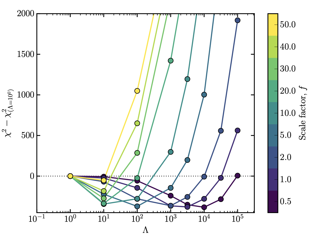
Regardless of whether you're using the \(L_1\) norm (LASSO) or \(L_2\) norm (Ridge), the regularisation strength \(\lambda\) will be different for every optimisation problem and every data set. You have to set it using some heuristic. Normally what people do is they split up their training data into two subsamples: 80% of the data that they will use for training, and 20% that they will use for validation. Then they will try different values of the regularisation parameter \(\lambda\), usually on a logarithmic grid from very small values to very high values (i.e., \(10^{-10}\) to \(10^{3}\)).The exact values will depend on your data set and you can do some back-of-the-envelope calculations to figure out what ranges of \(\lambda\) will actually matter for your problem. At each \(\lambda\) value they will optimise the weight coefficients \(\vec{w}\), and then they will evaluate the term \[ \textrm{cost} = \lVert{}\vec{Y} - \vec{Aw}\rVert{}^2 \] using only the 20% validation set. Note that we are not including the regularisation term here! We are only testing to see how well our regularised coefficients \(\vec{w}\) can describe the validation set data — data that it has not seen before! That is to say we use the regularisation parameter \(\lambda\) when 'training' the coefficients \(\vec{w}\), but when 'testing' on the validation set we do not include regularisation!

We then record that cost value and move to the next \(\lambda\) value to try. As you increase \(\lambda\) to higher values you will see something like a dip (see below), where at a given \(\lambda\) value the model is doing a better job at describing the validation data, and then at higher \(\lambda\) values it does a much worse job. From this we can set \(\lambda\) to be the point at the minima, and move on with our lives. This process is called cross-validation.Often you may want to do this process multiple times, with many random 20% subsets of the data. The exact split of 80/20 is arbitrary, but is probably reasonable for most problems.

\(\chi^2\) value of the validation set (minus an offset value) as a function of regularisation strength \(\lambda\) (Casey et al. 2014). Notice that the validation set \(\chi^2\) initially decreases with increasing \(\lambda\) — in that the regularised model is a better description for the validation set — before increasing very quickly. The scale factor here is irrelevant here.

Classification

Classification is the process of identifying which set of categories a new observation belongs to, based on a training set of observations with assigned categories.

There are many classification algorithms available. We will only cover some of these here:

Many of these algorithms are used in regression as well as clustering, and in other topics. That's because classification can be described as a regression problem where you round the output valueOr use some logistic function. into a classification bin. And many of these algorithms have similar names elsewhere, so don't get them confused!Examples include: logistic regression (is classification, not regression); \(k\)-nearest neighbours (is different from \(k\)-means), et cetera.

Classification performance by multiple different algorithms on three input data sets (source).

Logistic regression

Don't be fooled by the name: logistic regression is a classification algorithm, not a regression algorithm.I know. Logistic regression is used to predict the category of an observation, and it can provide probabilities of association to each category (i.e., 0.70 dog; 0.3 cat). You can have more than two categorial outputs, but here we will consider just two classifications.

Now consider some data to have two predictive features \(x\) and \(t\), and we are interested in classifing the output \(y\). Here \(y\) is a binary value (0 or 1) to indicate different classes of categories. Logistic regression assumes a linear relationship between the predictor variables \(x\) and \(t\) and the logarithm of the odds ratio \(\ell\) of the event that \(y = 1\) \[ \ell = \log\frac{p(y = 1)}{1 - p(y = 1)} = \beta_0 + \beta_1x + \beta_2t \] such that the probability that \(y = 1\), \(p(y = 1)\) is given by \[ p(y=1) = \frac{1}{1 + \exp\left[-\left(\beta_0 + \beta_1x + \beta_2t\right)\right]} \quad . \] You can see that in order to use this classifier we need to solve for the coefficients \(\beta_0\), \(\beta_1\), and \(\beta_2\). So we would use the input training set of \(x\), \(t\), and output labels \(y\) to do regression for the \(\beta\) coefficients, and then we can use the model to classify new data. It might be surprising to see that this classification algorithm is actually just regression! The trick is just the logistic function, which provides a smooth (and potentially rapid) transition between two numbers — integers, in this case!

Support vector machines

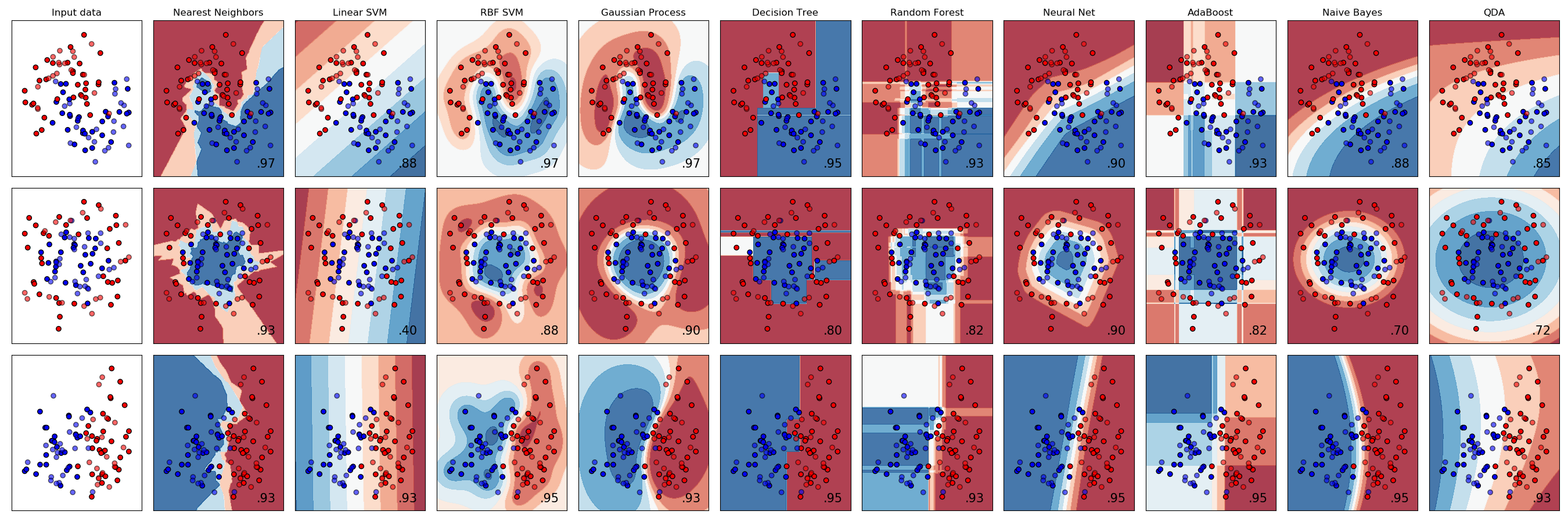
Support vector machines (SVMs) use training data to high-dimensional non-linear mapping between different categories in data space. Remember the kernel trick from Gaussian Processes where we were able to replace an inner product of infinite dimensional matrices with a kernel function that would reduce a non-linear mapping in a higher-dimensional latent space to a low-dimensional mapping in data space? SVMs use the same trick!

That means when using SVMs you have to decide what kernel you are going to use, just like if you were using a Gaussian Process. In general people either use linear kernels (Linear SVM), or a Gaussian radial basis function (RBF SVM) to capture smooth nearby groups of the same categories. What SVM does, exactly, is to use the kernel trick to define a non-linear boundary in data spaceWhich has been reduced from a linear boundary in a higher-dimensional latent space. to discriminate which category an object belongs to. The optimal boundary is one that maximises the separation between two classes. Take a look at the RBF SVM results from the comparison of clasification algorithms above. You can see that the RBF SVM is producing a nice, well-defined boundary in each case that defines whether an object came from the blue group, or the red group. This is a non-linear boundary that is learned directly from the training set data, and can be high-dimensional. Once this boundary is learned, new data can trivially be classified.

Just like Gaussian Processes, SVMs have hyperparameters (kernel parameters) that need to be optimised from the training set. Often these are found by running a grid search on the hyperparameter, where at each value of the grid search you evaluate the SVM's performance on a random subset of the data. SVMs are also a binary classifier, which means that to perform multi-class classifications you need to combine many SVM models together, each with a classification between one of two categories.

Random forests

Random forests are collections of decision trees, trained on subsets of the data, that provide an output classification based on a series of decision boundaries that are learned from the data.

A decision tree is used to define outcome classifications based on inputs, where there are multiple nodes in the tree. If you know something about your data you could define the nodes yourself, but in practice we want to learn the decision tree structure from the training data.

Consider the following decision tree that predicts survival outcomes for passengers on the RMS Titanic:

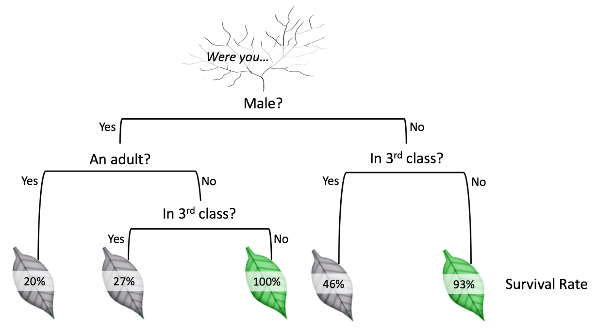
Decision tree to predict whether you'd survive the sinking of the RMS Titanic. [source]

Ideally we want the data to learn these optimal decision placementsOptimal in the sense that the position and flow of the nodes will best describe the data., but it can be difficult to find these. That's because there many be many input features, leading to a huge combinatorial problem to solve. And that means that decision trees can naively be extremely prone to over-fitting!

Random forests are collections of multiple decision trees, where each decision tree is only using a random subset of the features, and they only train on random samples of the data. These simple changes make random forests much more robust against over-fitting. Once a random forest has been trained you can use it to provide probabilistic classifications for multiple different classes (i.e., it is not just a binary classifier). They are extremely cheap to train and generally perform well on most problems.

Like SVMs, random forests will end up preferring to split data based on the boundaries (or set of sequential nodes) that separates the categories the most. Unlike SVMs, random forests are somewhat more interpretable because instead of just getting a boundary mapping in data space that describes whether an observation came from category 1 or 2, a random forest will be able to tell you which features are most important for predicting output classifications.

Summary

That was a broad introduction to the categories of classical machine learning. We included topics in supervised machine learning such as regression and classification, where you would have found that much of the regression is equivalent (or at least related) to the things you have done in earlier weeks. And classification is no more challenging, either: it is just regression with a logistic function!

In the next class we will cover dimensionality reduction and association. Dimensionality reduction is frequently used to compress massive data sets into things that are more manageable, and association became particularly famous by Netflix and Amazon through their recommendation systems.

Machine learning overview